When Equations Learn
An Intuitive Guide to the Math of AI
A. P. Rodrigues
Names: Rodrigues, A. P., author.
Title: When equations learn: an intuitive guide to the math of ai / by A. P. Rodrigues.
Description: First edition. | Passo de Torres, SC, Brazil : Published by the author, 2025.
Identifiers: ISBN 978-65-01-49720-4
Subjects: LCSH: Machine learning. | Artificial intelligence. | Neural networks (Computer science). | Computer science. | Mathematical models.
Classification: DDC 006.3
This book is lovingly dedicated…
To Eduardo, whose thoughtful bibliographic suggestion first pointed me toward the world of artificial neural networks.
To Professor Giovane, for his kindness and thoughtful attention — and to his brother, Vinícius.
To Daniel, for the conversations, insights, and counsel that proved invaluable.
To my dear friend and true father figure, Marcus Maia.
To Fabiano and Laura, whose gratitude blossomed into remarkable generosity.
To Professor Carmen Mandarino, with deep appreciation.
And to the One who created the neuron — whose design inspired the very birth of the Perceptron.
Preface
This is a freely distributed e-book, but if you wish, you can purchase a physical copy on the author’s website. This book is about artificial learning and how this gift is bestowed upon one of the most fundamental structures of all neural networks: the Perceptron.
This book presents the very basics of artificial learning in neural networks. Anyone can use it to get a first contact with the fascinating world in which machines are capable of learning almost anything and simulating important aspects of human intelligence, such as seeing, reading, speaking, understanding what another human being says, and several other very useful capabilities that have been increasingly within everyone’s reach.
The first two chapters of this book used to make up another book, not yet translated into English, I had titled "The Most Basic of the Basic of the Basics on Artificial Learning". The present work is a formidable expansion of the previous one. Although the treatment and scope of the content in this volume can still be said to be quite basic, it goes deeper into machine learning and shows how to endow deep models with the ability to learn.
Artificial learning is the admirable secret behind the wonders we see nowadays in the most well-known AIs, such as, for example, ChatGPT or Gemini. Without it, these truly monumental byproducts of technology would not have been possible. To build an artificial intelligence, it is not enough to just know how to write code in a good programming language like TensorFlow or PyTorch. These very languages are the result of having mastered the understanding of how to make a machine, a software, or an equation grasp and retain what we would like to teach them.
However, learning is usually encapsulated in methods, functions, classes, etc., of those languages, and an excellent programmer never needs to come into contact with them, if they do not wish to, in order to describe in code the structure they want to build. In this way, the most precious gift of all artificial intelligence, in my opinion, remains somewhat hidden.
The concealment, which is partly a side effect of the automation of the programmatic layers responsible for learning, is not without reason. It greatly expands the number of people who are able to bring an idea to life through artificial intelligence, even without ever having known anything about how artificial learning works.
Unfortunately, the mathematics that describes the phenomenon of learning is not normally taught before the higher education level in Brazil. And, although it is not difficult and can even be considered old mathematical knowledge, Differential Calculus and the derivative of functions end up being unknown to a large number of people.
This entire book is about deriving functions! The functions in question are Perceptrons! But, perceptrons are functions of a somewhat more elaborate type. They are not real-valued functions. They are functions that involve matrices and vectors!
Artificial learning, which is based on derivatives, is based on a technique known as backpropagation. It is the right way to derive a vector-type function that is compositionally deep. This book is about this. This is the main content of this book.
What I present in this work is not the only important thing you will need to know about machine learning, but it is the indispensable part! Without this central core, artificial learning and the pieces of artificial intelligence mentioned above would not exist.
I wrote this book much like I myself would have wanted to read about the subject when I began to study it. I tried to show what is, in my opinion, the most important thing within the set of the most important things, showing, for example, the equations for the Perceptron’s structure and for the functioning of learning, in an explicit and to-the-point manner, so that anyone knows exactly how to code them, in their preferred language, as soon as they glance at them. This was what I would have liked to have found when I began to study the subject. An elementary treatment, accessible to beginners, single-themed regarding learning, and that would go from conceptualization, through detailed description, and all the way to application. This book, as already mentioned, focuses heavily on the descriptive stage.
In appendix Fundamental Topics in Neural Network Learning Not Covered in This Book, you can find a list of important topics in machine learning that were not covered, or were only mentioned, or insufficiently addressed in the present version of this book. It serves as a good initial thematic reference for those who wish to continue broadening their knowledge on the subject.
Finally, there are some codes that I wrote for this book and that I have made available in the notebook that is in the GitHub repository. It is quite possible that in the future even more material will be pushed there.
Happy reading!
- Preface
- Introduction
- 1. Shall We Start with a Little Game?
- 2. The Basic Description
- 3. Artificial Learning
- 4. Multiple Layers
- 4.1. The Propagation of a Signal x Through the Network’s Layers
- 4.2. A 2-Layer Perceptron
- The Equation of a 2-Layer Perceptron
- The Error Function of a 2-Layer Perceptron
- The Rates of Change of the Error
- Derivative of the Error with Respect to the Layer 2 Weights
- Derivative of the Error with Respect to the Layer 2 Biases
- Derivative of the Error with Respect to the Layer 1 Weights
- Derivative of the Error with Respect to the Layer 1 Biases
- 4.3. A Multi-Layer Perceptron
- 4.4. The Error Function of a Multi-Layer Perceptron
- 4.5. The Derivative of the Error with Respect to the Weights of Any Given Layer
- 4.6. Practical Process for Updating Weights and Biases
- 4.7. Analyzing the Dimension of the Matrices for \( \frac{\partial E}{\partial W^l}\) and \( \frac{\partial E}{\partial b^l}\)
- 4.8. Updating the Weights and Biases
- 4.9. Giving Life to Equations
- 5. Training in Batches
- Appendix A: Norm on a Vector Space
- Appendix B: The Derivatives of \( y_i\)
- Appendix C: Derivative of Vector Functions
- Appendix D: Some Observations on the Gradient
- Appendix E: Outer Product
- Appendix F: Continuous Learning
- Appendix G: The Cost Function over a Matrix Domain is a Norm
- Appendix H: Fundamental Topics in Neural Network Learning Not Covered in This Book
Introduction
The Perceptron is probably the most basic of all neural network architectures. Although it can be used on its own in small projects and for simple tasks, it is present—one way or another—in the vast majority of today’s most well-known and celebrated AI systems, such as OpenAI’s ChatGPT or Google’s Transformer.
I present the most basic mathematical structure of the Perceptron—its operation and, most importantly, its learning—in a quick and straight-to-the-point manner. The theory I cover here is only what’s indispensable for the presentation—no detours—of this fundamental piece of modern artificial intelligence. Thus, this book does not address the history of the Perceptron, nor does it provide any general statistical or analytical treatment of the concepts presented, nor does it explicitly cover matrix theory or concepts of Linear Algebra, etc.
A few demonstrations are included in the Appendices for interested readers, but only because they help to clarify important and foundational points regarding what the author believes to be the most important topic in this entire field: how a neural network is able to learn.
Thus, this book was written more to exhibit and operate with the basic formulas that provide primary and solid understanding of the subject, rather than to rigorously prove or demonstrate them. My main intention is to present and describe, with clarity, what is most basic—mathematically speaking—so that this initial contact may guide the interested reader toward a firm understanding of the subject, useful as a foundation for further or more advanced reading later on.
Neural networks and the Perceptron in particular are human inventions that were initially modeled on what was understood about how neurons work. It is a model that faintly mirrors the behavior of a living natural object. As distant as the Perceptron model may be from what we now know about the immense complexity of a real neuron, the model is nonetheless an enormous success.
Being a human invention, its most fundamental mathematical modeling is elegant and beautiful in the very sense that it is extremely simplistic. The reader will likely get this impression at various points in the book, particularly in the first chapter and in the parts that specifically address its structure.
The content presented in this book—especially from Chapter 2 onward—was created with the goal of enabling readers to use or adapt the same concepts when studying other neural network architectures and deep learning systems.
Modern languages and frameworks, such as TensorFlow, are based on and make use of the concepts of vectors and matrices. Perhaps one of this book’s merits is in explicitly showing the matrix nature of the equations that describe the Perceptron—and especially those that describe its learning process.
From experience, we know that building neural networks using tools like TensorFlow does not require programmers to have the in-depth understanding I present here, simply because this understanding is embedded as a key component, in a way hidden beneath a high-level, intuitive, and easy-to-use interface. However, the clear and explicit representation of the differential and matrix-based nature underlying artificial learning will provide the reader with an exact understanding of the beauty and power that are usually hidden from the general public, who are dazzled by the luminous results of such knowledge applications.
1. Shall We Start with a Little Game?
Let’s start this book with a little game!
One that you will remember for the rest of this book’s reading. Perhaps, for the rest of your life.
We are going to "transform" a sequence of numbers into the number \( \pi=3.14\). That’s right, you read it correctly: we are going to transform!
"But which sequence of numbers?", you might ask. Any one will do, I would answer! You choose yours!
Mine will be 1, 2, 3, 4!
But, I could have chosen any other, like 3, 2, 1, 0, -1, -2; or \( \frac{1}{2}, \frac{3}{4}, 100, -\frac{1256}{100}, 8^3, 0.67,\sqrt{\frac{1}{6}}\), no matter what numbers are in the sequence or how many!
But, we will need another sequence of numbers! The one that will learn to transform [1, 2, 3, 4] into the single number 3.14! Yes, we need another sequence! And this second sequence is the most important sequence.
This other one can also start with any numbers, but it helps a lot if, initially, it only has small numbers close to zero! And, this other sequence must have the same number of elements as the first one.
I chose the following: [0.9, 1.5, -0.1, 0.3].
I cannot overstate the importance of this sequence! It will hold the learning responsible for transforming [1, 2, 3, 4] into 3.14.
The four initial values that we see in the learning vector are not so important yet, but the four values we obtain at the end, when we finish playing, those are the most important ones!
To start, let’s combine [1, 2, 3, 4] with [0.9, 1.5, -0.1, 0.3]! That’s right! We are going to combine! And, combine linearly! In other words, we are going to treat these sequences as if they were vectors, and we are going to multiply one vector by the other, and see what happens:
Now, 4.8 is not yet 3.14, and not even close enough to 3.14!
So, we have to do something about it!
The initial version of our learning sequence has a negative number. It can be seen in the first line of 1. What if we tweak this number so that, in the end, we get a value smaller than 4.8 and closer to 3.14?!?
What could we do with -0.1 to transform 4.8 into a value closer to 3.14?
Notice that to get to 3.14 from 4.8, we could do 4.8 - 1.66! But how can we tweak the values of the vector [0.9, 1.5, -0.1, 0.3] to get the difference, -1.66, that we need in the final value?
Let’s "take a guess," as they say, and if it’s still not right, we’ll adjust it later!
So, let’s do the following: let’s change -0.1 to -0.3; and let’s also change 1.5 to 0.97.
Thus, our initial learning vector is already learning (or trying to!), as it went from [0.9, 1.5, -0.1, 0.3] to [0.9, 0.97, -0.3, 0.3]!
And, just look!
Notice that we only changed two of the four numbers in our initial learning vector. But we could have changed all of them!
What exactly did we do to those two values of the original vector? We subtracted 0.53 from 1.5 to get 0.97 in the second position, and we added -0.2 to -0.1 to get -0.3 in the third position. I found the -0.53 and the -0.2 through repeated attempts. I observed the effect that each attempt had in getting closer to or further from the desired result, until I found values increasingly closer to 3.14!
In this small example, we have just used our real intelligence to do something similar to what artificial intelligence models routinely do when they are learning!
They make small adjustments to a multitude of numbers distributed across many vectors. These vectors are usually very large, and the adjustments are made many, many times so that, each time, the small changes contribute to bringing the entire model to a response closer to the response that one wants the model to produce.
This book is about the beautiful, ingenious, and precise way in which such adjustments are calculated and applied!
Notice that we could have made adjustments to several vectors at the same time, each producing its own result! Our natural intelligence would find it tiring to deal with numbers in several vectors at a minute and tedious level of detail! But that is exactly what artificial intelligence models can do for us!
In fact, these models, also called artificial neural networks, do much more than just approximate numbers. They are capable of approximating curves and surfaces, and in general, they can approximate or map datasets of a complicated nature that describe, among other things, characteristics of human intelligence, such as vision, hearing, or speech.
I mentioned the concept of mapping above. In our little game, we created a mapping! A very simple one, but functional nonetheless. The mapping we created uses the learning we stored in the vector [0.9, 0.97, -0.3, 0.3] to create a functional relationship between one vector, [1,2,3,4], and the number 3.14, so that we can symbolize this functional relationship, y=f(x), like this: \( f(x)=[0.9, 0.97, -0.3, 0.3] \cdot x\), so that \( f([1,2,3,4])=[0.9, 0.97, -0.3, 0.3] \cdot [1,2,3,4]=3.14\)!
Get ready, because in the rest of the book we will see much more about these fabulous mappings and how to apply automatic mathematical optimization processes to them that will make artificial learning a true child’s play.
1.1. Giving Life to Equations
The Initial Game in Code
To start getting familiar with implementing the ideas, let’s replicate the "little game" from our Introduction using Python and the NumPy library.
The code below declares the two vectors we used: the input vector x (the data we want to transform) and the weight vector w (the "knowledge" of our equation). We will see the result of the initial linear combination, the "learning leap" with the already adjusted weights, and the formalization of our functional relationship into a function f(x).
Each line of code mirrors a step from our little game.
 1import numpy as np
 2
 3# --- 1. The Starting Point ---
 4
 5# The input vector we want to "transform".
 6x = np.array([1, 2, 3, 4])
 7
 8# The initial weight vector, our still-incorrect "knowledge".
 9# In the book, we call this the "learning sequence".
10w_inicial = np.array([0.9, 1.5, -0.1, 0.3])
11
12# The linear combination (dot product) we did on paper.
13resultado_inicial = np.dot(x, w_inicial)
14
15print(f"Input Vector (x): {x}")
16print(f"Initial Weights (w_inicial): {w_inicial}")
17print(f"Initial Result (x . w_inicial): {resultado_inicial:.2f}")
18print("---")
19
20
21# --- 2. The Learning Leap ---
22
23# The weights after our "magical" adjustment, as we did in the game.
24# This is the final "knowledge" that the equation has learned.
25w_final = np.array([0.9, 0.97, -0.3, 0.3])
26
27# The new combination with the weights that have "learned" the task.
28resultado_final = np.dot(x, w_final)
29
30print(f"Final Weights (w_final): {w_final}")
31print(f"Final Result (x . w_final): {resultado_final:.2f}")
32print("---")
33
34
35# --- 3. Formalizing the Learning ---
36
37# We create a function f(x) that encapsulates the learned knowledge.
38# This function is our final "model", ready to be used.
39def f(input_vector):
40    # The learned weights are "stored" inside the function.
41    learned_weights = np.array([0.9, 0.97, -0.3, 0.3])
42    return np.dot(input_vector, learned_weights)
43
44# Using the function to prove that the transformation works.
45pi_calculado = f(x)
46
47print(f"Executing the learned function f(x):")
48print(f"f({x}) = {pi_calculado:.2f}")
49
50if np.isclose(pi_calculado, 3.14):
51    print("\nSuccess! Our equation has learned to calculate π!")
The Extended Game: Simultaneous Adjustment
Now, let’s extend the game. What if we wanted a single set of "neurons" to learn to perform several tasks at the same time?
In the example below, we will use the same logic, but with a weight matrix W. Each row of the matrix W will act as a separate "neuron," responsible for a different transformation. Our goal is to adjust the three rows of W so that, from a single input vector x, our model simultaneously calculates approximations for three famous constants:
-
π (Pi) ≈ 3.14
-
e (Euler’s Number) ≈ 2.71
-
h (Planck’s Constant, scaled value) ≈ 6.63
The flow is the same: we will show the result with the initial (random) weights and then the result with the final, "mysteriously" adjusted weights, showing the power of simultaneous adjustment.
 1import numpy as np
 2
 3# --- 1. Defining the Targets and Input ---
 4
 5# Our targets: the three constants we want the network to learn to generate.
 6# Note: The value of h (6.626e-34) has been scaled to 6.63 for didactic purposes.
 7alvos = np.array([3.14, 2.71, 6.63]).reshape(3, 1) # Column vector of desired responses 'z'
 8
 9# We will use the same input vector 'x' for all tasks.
10x = np.array([1, 2, 3, 4]).reshape(4, 1) # Column vector for input
11
12# --- 2. The Starting Point with Random Weights ---
13
14# The initial weight matrix W. Each row is a "neuron" with 4 weights.
15# 3 neurons (one for each constant), 4 weights each. Matrix shape: (3, 4).
16np.random.seed(42) # For reproducible results
17W_inicial = np.random.randn(3, 4) * 0.5 # Small random numbers
18
19# The initial linear combination using matrix multiplication (W . x)
20# The result is a vector of 3 elements, one per neuron.
21resultado_inicial = np.dot(W_inicial, x)
22
23print("--- Initial State ---")
24print(f"Input Vector x:\n{x.T}")
25print(f"\nInitial Weight Matrix W_inicial:\n{W_inicial}")
26print(f"\nInitial Result (W_inicial . x):\n{resultado_inicial}")
27print("As expected, the initial result is random and does not resemble our targets.")
28print("-" * 25)
29
30
31# --- 3. The Simultaneous Learning Leap ---
32
33# Here is the "magical" weight matrix after the adjustment.
34# Each row has been adjusted for its respective task.
35# (These values were pre-calculated so that the result is correct)
36W_final = np.array([
37    [0.9, 0.97, -0.3, 0.3],      # Row that "learned" to calculate Pi
38    [0.1, 0.5, 0.8, -0.1525],   # Row that "learned" to calculate 'e'
39    [1.0, 2.0, 0.9, -0.2425]    # Row that "learned" to calculate 'h'
40])
41
42# The new combination with the weight matrix that has "learned" the three tasks.
43# Note, below, that the final results are very close to the desired targets. Although we could
44# have obtained the exact values for π ≈ 3.14, e ≈ 2.71, and h ≈ 6.63 by adequately
45# manipulating the weights of W_final in more adjustment steps, this is what is normally
46# obtained numerically in real projects: very good approximations.
47resultado_final = np.dot(W_final, x)
48
49print("\n--- Final State (After Learning) ---")
50print(f"Final Weight Matrix W_final:\n{W_final}")
51print(f"\nFinal Result (W_final . x):\n{resultado_final}")
52print(f"\nDesired Targets:\n{alvos}")
53
54# Verifying the success
55if np.allclose(resultado_final, alvos, atol=0.01):
56    print("\nSuccess! Our weight matrix has learned to perform three tasks simultaneously!")
2. The Basic Description
Among artificial neural networks, the perceptron is the simplest.
The Perceptron is, so to speak, the building block of most neural network models.
Its structure is simple and easy to understand.
Mathematically, the Perceptron is an equation that learns.
But what does the Perceptron’s equation learn? Anything! It learns to provide the answers we want it to give for the elements of any given set of data or information. From this perspective, the Perceptron learns to create a point-to-point mathematical relationship between a set of data, \( D\), and another set of desired responses, \( Z\). This relationship takes the functional form \( P: D\longrightarrow Z\) and acts as the equation \( P(d)=z\) between specific points.
2.1. Weights and Biases, or Trainable Parameters
The Perceptron is based on a matrix of trainable parameters, \( W\), and also a vector of other trainable parameters, \( b\).
and
These parameters are called trainable because they change during the perceptron’s training, mysteriously accumulating the network’s learning until they reach an optimal value. At that point, the network is ready to perform the task it was created for.
The elements of the matrix \( W\) are the perceptron’s weights, while the vector \( b\) is the bias. The elements of \( b\) are the biases for each neuron.
To put it very simply and directly, the number of rows in \( W\) is the number of neurons in the Perceptron, and the number of columns is the number of weights for each neuron. All neurons (in the same layer) have the same number of weights.
I referred to the perceptron as the building block of most neural networks. Neural networks are built with basic structures called layers, and the Perceptron is this layer in a vast majority of network architectures. Furthermore, the Perceptron itself can have layers, as we will see in Chapter 3.
Note that if the Perceptron consisted of a single neuron, then the matrix \( W\) representing this layer would, in fact, be a row-vector! That is, \( W\) would be a \( 1\times m\) matrix:
Just to give an example, as incredible as it may seem, even Deep Learning projects with more complex and deep architectures that perform binary classification are likely using a Perceptron with a single row of weights as their final layer. This would be the case for a network whose goal is to read bone x-rays and determine whether they indicate fractures. Such a well-developed network could be trained to identify fissures or fractures that are difficult for the human eye to detect.
2.2. The General Form of the Perceptron
A perceptron, like any other neural network, is created to perform a task. It must learn to perform its task. It must produce a result, \( z\), that corresponds to each element, \( x\), both in a set of data or information, \( D\). We say that \( D\) is a set of vectors or tensors and that the perceptron is trained on this set. We will talk more about \( D\) when we get to Section Training.
If \( x\in D\) is one of the training vectors, then the perceptron’s response, \( y\), to this vector is:
The vector \( x\) is one of the perceptron’s inputs, and \( y\) is the corresponding output.
Any of the expressions in (6) are sometimes simply called the perceptron’s linearity.
2.3. Two Alternative Representations
Below, I will briefly present two alternative ways the Perceptron can be represented. The reader may encounter these in other books, and knowing they exist can broaden one’s ability to manipulate the mathematical tools that describe and model it. I include them here in passing, but we will not use them in this book.
The \( xW\) Form of the Matrix Product
Note that the first equation of 6 could have been written with the vector \( x\) multiplying the matrix \( W\) from the left, like this:
in which case the vector \( x^T\) would be a row-vector, the columns of \( W^T\) would be the Perceptron’s neurons, while the number of rows in \( W^T\) would be the number of weights in each neuron.
Weights and Bias in the Same Matrix
We can embed the bias vector of each layer into its respective weight matrix, making it the last column of these matrices. This possibility is already present in the Perceptron’s equations. Consider, for example, the third equation in 6 and notice that it can be rewritten as follows:
with \( b_i=w_{i(m+1)}\) and with \( x_{m+1}=1\).
Now, note that the second equation in 8 is the same as:
This way, we would only need to embed the scalar unit as the last position of each incoming vector, \( x\), so that it now has \( m+1\) elements.
In this way, the equation above is simply:
2.4. Activation Functions
It is extremely common to pass each of the values of \( y\) to the same activation function. This activation function is also known as a "non-linearity," because it "breaks," in a way, the linear behavior produced in 6. It can take one of several commonly used forms. For now, let’s just designate it with a symbol: \( a\). Thus, in its most general form, the single-layer perceptron is:
This last expression might seem a bit confusing at the moment, perhaps because of the expressions inside the brackets, but don’t be alarmed. It displays the mathematical symbols that mirror the conceptual structure of a single-layer Perceptron. It also shows how the vector \( x\) is "absorbed" and processed by the network. The vectors \( W_i\) are the rows of \( W\) and the scalars \( b_i\) are elements of \( b\). See how the vector \( x\) is processed by each of the rows of \( W\). The equation shows how the signal \( x\) "flows" through the perceptron until it is transformed into its response, \( P\).
Try to firmly grasp the fact that \( a\) is a vector and that its elements are functions whose independent variables are, respectively, the elements of the vector \( y\). In the Subsection below, I have placed a table with some well-known and commonly used activation functions.
Some Activation Functions
The table below displays some of the most well-known activation functions. They are shown with the notation we use throughout the book, revealing their nature as real-valued functions of a real domain, with the exception of the Softmax function. The Softmax function uses all components of a linearity vector to generate a percentage relative to the \( i\)-th component.
| Name | Formula |
|---|---|
Sigmoid |
\( a_i(y_i)=\frac{1}{1+e^{-y_i}}\) |
Hyperbolic Tangent |
\( a_i(y_i)=\tanh(y_i)\) |
Softmax |
\( a_i(y) = \frac{e^{y_i}}{\sum_{k=1}^{n}e^{y_k}}\) |
ReLU |
\( a_i(y_i) = \max\{0,y_i\}\) |

2.5. Training
We have already said that a perceptron must learn to perform a certain task and that it is trained on a set of data or information, \( D\). This set can be considered a set of ordered pairs, \( (x,z)\in D\), such that \( z\in Z\subset D\) and \( x\in X\subset D\) are, respectively, the set of desired responses and the set of vectors representing any domain of things we are interested in relating to the desired responses.
We have already seen that \( x\) is a vector. The second component of the ordered pair, \( (x,z)\), is the response we want the perceptron to learn to give to the input vector \( x\). The ordinate \( z\) can be a scalar number, a vector, a matrix, or a tensor. This will depend on how we mathematically encode the task. In this book, our desired responses, \( z\), will only be scalars or vectors.
Initially, the perceptron gives some arbitrary response, \( P\), to the vector \( x\). Throughout the training, this response gets closer to the correct or desired response, \( z\). We check this approximation with a Cost Function, which we will denote with the symbol \( E\) (we will see more about it in Section The Cost Function), which tells us how far or how close \( P(x)\) is from the desired response \( z\). Throughout the training, the value of the Cost Function decreases because \( P(x)\) becomes increasingly close to \( z\). Our goal during training is to make the error go to zero, meaning that the equality \( P(x)=z\) becomes true, or almost true, as a sufficiently small error is usually enough.
From a certain point of view, this entire book is about how to reintegrate into the Perceptron, during training, the information contained in the error, \( E\), to make the Perceptron more accurate in its task. That is, to create the relationship we desire, \( P(x_i)=z_i\).
There are several functions that can be used as a cost or loss function. The choice depends on the project and sometimes on the preference of the person training the network. In Section Some Cost Functions, there is a table with some useful and commonly used cost functions. The important thing to know is that the Cost Function, whatever it may be, must comply with the mathematical definition of a norm. This is a topic we won’t delve into in this book, but the interested reader can find the definition in Appendix Norm on a Vector Space, along with a small proof that if a norm is zero, then its argument must also be zero.
We will see in Section Updating the Trainable Parameters that the process we will use to approximate \( P(x)\) and \( z\) is based on the gradient of the Error Function. This process, called Gradient Descent or Stochastic Gradient Descent, gradually indicates the direction of the lowest value of \( E\) and, thus, also indicates the path to a smaller separation between \( P\) and \( z\).
We can say that the Perceptron is a mapping that learns to give an appropriate response \( z\) to each \( x\) in a learning process that is carried out over one or several training sessions. Usually, several! In a training session, the Perceptron receives all the elements \( x\) from \( D\), one after the other, and for each \( x\), the corresponding \( P(x)\) is calculated. After that, the error function is calculated on \( P(x)\) and \( z\), so we can express it as: \( E(P,z)\). As many training sessions are performed as necessary to make \( E(P,z)\) sufficiently close to zero. This is the reason for requiring the Error or Cost Function to be a norm, because then, when \( E(P,z)\longrightarrow 0\), it will also be true that \( P-z\longrightarrow 0\), meaning the network’s response is becoming equal to the desired response.
3. Artificial Learning
3.1. Optimization
Artificial learning is an optimization process.
What is optimized in artificial learning? A function that is usually called a Cost Function, Loss Function, or even Error Function! I personally call it, in this context of artificial learning, a Pedagogical Function, since it measures how far the Perceptron’s response is from the desired response, and by this means, we know if the network is learning or not. It is from the derivation of the Loss Function that learning happens.
Anyone who has ever derived a function to then find its maximum or minimum is in a perfect position to understand how artificial learning happens.
Learning occurs in one or more training sessions, where the Perceptron’s trainable parameters are repeatedly updated (See Section Training). These parameters are updated at each step of the training, that is, after each training batch is presented to the network. We will see more about training in batches in the chapter Training in Batches.
The description of how artificial learning happens is the most important and interesting part of neural networks in this author’s opinion. Without this, there is no machine learning.
3.2. The Cost Function
When we go to school, our learning is measured by assessments. The learning of neural networks is also measured by performance evaluations.
The Perceptron’s school is the training session.
Just as a final school grade is obtained from a formula, neural networks also use formulas that "grade" their performance.
In the case of neural networks, such formulas are known as cost functions, loss functions, or error functions. In this book, I refer to them much more often as error functions. They, in fact, measure the error made by the network when trying to predict a response to a corresponding input.
The error function can have several forms, but I will not address any specific form now, as we are interested in how its general form fits into the learning formulas. For now, we will just symbolize any error function with the letter \( E\). In Subsection Some Cost Functions, right below, you can find a table with some cost functions.
There is much to say about \( E\), but for now, let’s stick to the operational aspects that make it possible for the perceptron to learn.
The function \( E\) takes the Perceptron’s output as its argument. So,
But, you see, the perceptron’s output depends on its trainable parameters, meaning \( E\) also depends on the weights and bias. So, it is more common to write:
This notation is very useful because the perceptron’s learning depends on the derivative of \( E\) with respect to its weights and bias.
Here, we need to consider the compositional structure of the error function,
and keep in mind that \( a\) and \( y\) are vectors—the data from 6 and 11—and that \( E\) is a real-valued function.
Some Cost Functions
Below are some of the most well-known Cost Functions (with a vector domain).
| Name | Formula |
|---|---|
Mean Squared Error |
\( E=\frac{1}{n}\sum_{i=1}^n(a_i-z_i)^2\) |
Mean Absolute Error |
\( E=\frac{1}{n}\sum_{i=1}^n \begin{vmatrix}a_i-z_i\end{vmatrix}\) |
Cross-Entropy |
\( E=-\frac{1}{n}\sum_{i=1}^n z_i\cdot \log a_i\) |
Binary Cross-Entropy |
\( E=-\frac{1}{n}\sum_{i=1}^n \begin{bmatrix}z_i\cdot \log a_i+(1-z_i)\cdot \log (1-a_i)\end{bmatrix}\) |
3.3. Gradient of the Error with Respect to W
Let’s calculate the derivative of the error function with respect to the Perceptron’s weights. This derivative is also known as the gradient of the Error.
We know that \(\frac{\partial E}{\partial a}\) is the gradient of \( E\) with respect to the activation vector \( a\), because \( E\) is a real-valued function with a vector domain. Thus, \(\frac{\partial E}{\partial a}=\nabla_a E\).
The derivative \(\frac{\partial a}{\partial y}\) generates a matrix. This comes from the fact that both \( a\) and \( y\) are vector functions. See appendix Derivative of Vector Functions for more details on derivatives of vector functions.
The derivatives \(\frac{da_i}{d y_i}\) cannot yet be calculated or fully reduced. We don’t yet have any definite form for a. This will happen when we are dealing with specific examples or architectures.
If we analyze equation 11, we will see that each \( a_i\) depends only on \( y_i\). Therefore, we must have \(\frac{d a_i}{d y_j}=0\) if \( i \ne j\). Consequently, \(\frac{\partial a}{\partial y}\) will be a diagonal matrix. The elements, \(\frac{da_i}{d y_i}\), of this diagonal matrix will depend on the specific form of \( a\).
The differential \(\frac{\partial y}{\partial W}\) has the form of a column-vector with \( n\) elements. However, these elements are, in turn, \( n\times m\) matrices.
Now, notice that each element \( i\) of the column-vector on the right side of 16 is the derivative of a real-valued function whose arguments coincide only with the \( i\)-th row of \( W\). These real-valued functions are defined in equation 6, from which we know that \( y_i(W_i)=\sum_{j=1}^{m} w_{ij}x_j +b_i\) (See Appendix The Derivatives of \( y_i\) to review the procedure for deriving this equation). Therefore, the elements of the column-vector are matrices with null entries, with the sole exception of their \( i\)-th row.
Column-vectors or row-vectors of matrices will appear many times in this presentation. This is due to the fact that we are deriving the error, \( E\), with respect to the entire weight matrix at once.
Thus, the formula 15, which calculates the partial derivative of the perceptron’s error \( E\) with respect to its weights \( W\), is:
3.4. Gradient of the Error with Respect to the bias b
We now need to calculate the derivative of E with respect to the bias vector, \( b\).
From 6, we see that the biases are embedded at the deepest level of the perceptron, along with the weights.
Before, we considered the error as a function of only the weights. Now, let’s consider it as a function of only the biases.
Based on the calculations we’ve already done in the previous section, we can very simply write:
If necessary, see Appendix The Derivatives of \( y_i\) for more considerations on the calculation of \(\frac{\partial y}{\partial b}\).
3.5. Some Cost and Activation Functions and Their Derivatives
| Name | Formula | Derivative \(\left(\frac{d a_i}{d y_i}\right)\) |
|---|---|---|
Sigmoid |
\( a_i(y_i)=\frac{1}{1+e^{-y_i}}\) |
\(\begin{aligned} &\frac{e^{-y_i}}{(1+e^{-y_i})^2}\\ &\text{or}\\ &a_i(1-a_i) \end{aligned}\) |
Hyperbolic Tangent |
\( a_i(y_i)=\tanh(y_i)\) |
\(\begin{aligned} &1-tanh^2 y_i\\ &\text{or}\\ &1-a_i^2 \end{aligned}\) |
Softmax |
\( a_i(y) = \frac{e^{y_i}}{\sum_{i=1}^{n}e^{y_i}}\) |
\(\begin{aligned} &\frac{e^{y_i}}{\sum_{j=1}^{n}e^{y_j}} \left( 1- \frac{e^{y_i}}{\sum_{j=1}^{n}e^{y_j}} \right )\\ &\text{or}\\ &a_i(1-a_i) \end{aligned}\) |
ReLU |
\( a_i(y_i) = \max\{0,y_i\}\) |
\(\max\{0,1\}\) |
| Name | Formula | Derivative \(\left(\frac{d E}{d a_i}\right)\) |
|---|---|---|
Mean Squared Error |
\( E=\frac{1}{n}\sum_{i=1}^n(z_i-a_i)^2\) |
\( -\frac{2(z_i-a_i)}{n}\) |
Mean Absolute Error |
\( E=\frac{1}{n}\sum_{i=1}^n \begin{vmatrix}a_i-z_i\end{vmatrix}\) |
\(\begin{equation*} \begin{aligned} &\frac{1}{n} \frac{a_i-z_i}{\begin{vmatrix}a_i-z_i\end{vmatrix}}\\ &\text{or}\\ &\frac{1}{n} \begin{cases} 1 & \text{if}\ \ a_i>z_i \\ -1 & \text{if}\ \ a_i<z_i \\ \nexists & \text{if}\ \ a_i=z_i \end{cases} \end{aligned} \end{equation*}\) |
Cross-Entropy |
\( E=-\frac{1}{n}\sum_{i=1}^n z_i\cdot \log a_i\) |
\( -\frac{z_i}{na_i}\) |
Binary Cross-Entropy |
\( E=-\frac{1}{n}\sum_{i=1}^n \begin{bmatrix}z_i\cdot \log a_i +(1-z_i)\cdot \log (1-a_i)\end{bmatrix}\) |
\(\frac{a_i-z_i}{a_i(1-a_i)}\) |
3.6. Updating the Trainable Parameters
Finally, we’ve arrived where we wanted: \( \frac{\partial E}{\partial W}\) and \( \frac{\partial E}{\partial b}\) will be used to update the perceptron’s weights and bias. The process where this is done is called backpropagation and is based on the Stochastic Gradient Descent technique. This technique, in turn, is based on the fact that \( \frac{\partial E}{\partial W}\) is a gradient vector and, therefore, always points in the direction of the greatest rate of change of \( E\). Consequently, its negative, \( -\frac{\partial E}{\partial W}\) (see formulas 21 and 23), will point in the direction of the smallest variation. I won’t go into further detail on this point here, but the interested reader can find a few other interesting and pertinent observations about our use of it in Appendix Some Observations on the Gradient. I will just mention that the aforementioned negative sign is very important. If you have ever coded this formula, say in Python or TensorFlow or any other language or framework, to train a Perceptron, but mistakenly used a positive sign instead of a negative one, you may have noticed that the error made by the Perceptron actually only increases instead of decreasing!
At this moment, we have everything necessary to present the formula that allows learning to happen. This formula has a simplicity and beauty that is only matched by its power to make the Perceptron’s learning possible.
During a training session, the Perceptron’s weights are updated many times. Each update happens at a moment, \( t\), of the training. As the training evolves, the weights are altered in search of better performance, that is, in search of a lower cost, \( E\). At a given moment, \( t\), of the training, the perceptron has the weight matrix \( W_t\), which is updated by adding \( \Delta W_t\). The result becomes the new current weight matrix of the Perceptron, \( W_{t+1}\).
where
The symbol \( \eta\) is called the learning rate. It is a parameter whose importance lies in dictating the pace of the training, as it allows for adjusting the "speed" of the training. However, it is difficult to know what the optimal speed is for each step of a neural network’s training, although there are general guidelines and useful calculation methods, which we will not discuss at this time. It is a somewhat delicate parameter to handle, as are other defining parameters of neural networks. In practice, small values like \( \eta=0.01\) or \( \eta=0.001\) are always used as a first alternative. Other approaches alter the value of \( \eta\) throughout the training so that its value decreases as the training progresses.
The bias update is done with formulas very similar to those for updating the weights:
where
3.7. Giving Life to Equations
Artificial Learning: A First Example.
This notebook implements our first functional Perceptron in its simplest possible form: a single layer with a single neuron. We will use only Python and NumPy to see the theory from Chapters 1, 2, and 3 in its purest form.
The objective is to apply backpropagation to a real and quite rudimentary image classification problem. As our architecture is the simplest that exists, we will see how the general learning equation 17 simplifies in a beautiful and intuitive way. The calculation of the weights' gradient (∂E/∂W), for example, will not have that clumsy column-vector of matrices, as we will see.
 1import numpy as np
 2import matplotlib.pyplot as plt
 3import requests
 4from PIL import Image
 5from io import BytesIO
 6
 7# Function to download and prepare an image from a URL
 8def download_and_prepare_image(url):
 9    response = requests.get(url)
10    img = Image.open(BytesIO(response.content))
11    img = img.convert('L')
12    img_array = np.array(img) / 255.0
13    img_array = np.where(img_array > 0.7, 1, 0)
14    return img_array.flatten()
15
16# URLs of the "little faces" images
17base_url = 'https://raw.githubusercontent.com/aleperrod/perceptron-book/2e9af4436dd7317ea18fbcae583429cccc944ef0/carinhas/'
18urls = [
19    base_url + 'gross1.png', base_url + 'gross2.png', base_url + 'gross3.png',
20    base_url + 'thin1.png',  base_url + 'thin2.png',  base_url + 'thin3.png'
21]
22
23X_train = np.array([download_and_prepare_image(url) for url in urls])
24z_train = np.array([0, 0, 0, 1, 1, 1])
25
26# Test images
27url_teste_thin = base_url + 'thin4.png'
28url_teste_gross = base_url + 'gross4.png'
29x_teste_thin = download_and_prepare_image(url_teste_thin)
30x_teste_gross = download_and_prepare_image(url_teste_gross)1# Visualizing our training data
2fig, axes = plt.subplots(1, 6, figsize=(15, 3))
3for i, ax in enumerate(axes):
4 ax.imshow(X_train[i].reshape(20, 20), cmap='gray') # Reshape error, corrected to 20x20
5 ax.set_title(f"Class: {'Gross' if z_train[i] == 0 else 'Thin'}")
6 ax.axis('off')
7plt.suptitle("Sample of the Training Data ('Little Faces')", fontsize=16)
8plt.show()
Step 2: Defining the Tools (Functions)
As we are building everything "by hand," we define our tools as separate functions. Note that, as our Perceptron has only one neuron, the output P and the error E are single values (scalars), which simplifies their derivatives.
 1# Activation Functions and their derivatives
 2def sigmoid(y):
 3    return 1 / (1 + np.exp(-y))
 4
 5def sigmoid_derivative(a):
 6    return a * (1 - a)
 7
 8# Cost Function (Mean Squared Error) and its derivative
 9# z and P are scalars here
10def mean_squared_error(z, P):
11    return (z - P)**2
12
13def mean_squared_error_derivative(z, P):
14    return 2 * (P - z) # Keeping the factor of 2 for fidelity to the formal derivative
15
16# Function to initialize the parameters of our neuron
17def initialize_parameters(input_dim):
18    # W is a 1D vector (not a matrix) with 400 weights.
19    W = np.random.randn(input_dim) * 0.01
20    # b is a single number (scalar)
21    b = 0.0
22    return W, b
Step 3: Training "by Hand" (Example by Example)
This is the heart of our notebook. The training loop implements the theory of artificial learning. For each image x and its label z, the process is:
-
Forward Pass: We calculate the output
P, which in this case is a single number. -
Backpropagation: We calculate the gradients. Here lies the beauty of the simplification:
-
The error "delta"
dE/dyis a scalar, as there is only one linearity,y. -
The gradient of the weights,
dE/dW, is calculated by multiplying this scalar delta by the input vectorx. The equation∂E/∂W = (∂E/∂a * ∂a/∂y) * xmanifests here. The expression 17 simplifies because, in this example, the weight matrixWreduces to a row-vector!
-
-
Update: We adjust
Wandbusing the calculated gradients.
 1# --- Hyperparameters and Initialization ---
 2learning_rate = 0.1
 3epochs = 30
 4W, b = initialize_parameters(X_train.shape[1])
 5
 6cost_history = []
 7
 8print("Starting the training in Python/NumPy (corrected version)...")
 9for i in range(epochs):
10    total_epoch_cost = 0
11    # The inner loop iterates over each example individually
12    for x, z in zip(X_train, z_train):
13
14        # --- 1. Forward Pass ---
15        # y = W . x + b (dot product between two vectors -> scalar)
16        y = np.dot(W, x) + b (1)
17        # P = a(y) (activation on a scalar -> scalar)
18        P = sigmoid(y) (2)
19
20        # --- 2. Cost Calculation ---
21        cost = mean_squared_error(z, P)
22        total_epoch_cost += cost
23
24        # --- 3. Backpropagation (with scalars) ---
25        # Initial delta: dE/dy = dE/dP * dP/dy (product of scalars)
26        dE_dP = mean_squared_error_derivative(z, P)
27        dP_dy = sigmoid_derivative(P)
28        dE_dy = dE_dP * dP_dy
29
30        # Gradients of the parameters
31        # dE/dW = dE/dy * d(y)/dW = dE/dy * x
32        # This is the simplified form! It is the multiplication of a scalar (dE_dy) by a vector (x).
33        dE_dW = dE_dy * x
34        # dE/db = dE/dy * d(y)/db = dE/dy * 1
35        dE_db = dE_dy
36
37        # --- 4. Parameter Update ---
38        W -= learning_rate * dE_dW
39        b -= learning_rate * dE_db
40
41    # End of epoch
42    average_cost = total_epoch_cost / len(X_train)
43    cost_history.append(average_cost)
44    if (i + 1) % 5 == 0:
45      print(f"Epoch {i + 1}/{epochs} - Average Cost: {average_cost.item():.6f}")
46
47print("Training finished!")| 1 | Here, the linearity is \( y=W\cdot x+b\), which for our present case is \( y=\begin{bmatrix}w_{1}&,\dots , & w_{400}\end{bmatrix}\cdot\begin{bmatrix} x_1 , \dots , x_{400}\end{bmatrix}^t+b\) (the superscript \( t\) denotes the transpose from row to column), which in turn is equivalent to \( y=w_{1}x_1+\dots +w_{400}x_{400} +b\). |
| 2 | We return the sigmoid activation function \( P=a(y)=\frac{1}{1+e^{-y}}=\frac{1}{1+e^{-(W\cdot x+b)}}=\frac{1}{1+e^{-(w_{1}x_1,\dots , w_{400}x_{400} +b)}}\). |
Step 4: Analyzing the Training Results
One thing is to run the training, another is to know if it worked. The graph below shows the evolution of the average cost over the epochs.
A descending curve is the sign we are looking for: it indicates that the Perceptron was, with each pass through the data, adjusting its weights and becoming progressively better at its task, meaning the error was decreasing.
1# Plot the cost function graph to see if the network learned
2plt.figure(figsize=(10, 6))
3plt.plot(cost_history, marker='o', linestyle='-')
4plt.xlabel("Epoch")
5plt.ylabel("Average Error / Cost")
6plt.title("Error Evolution During Training (Python/NumPy)")
7plt.grid(True)
8plt.xticks(np.arange(len(cost_history)), np.arange(1, len(cost_history) + 1))
9plt.show()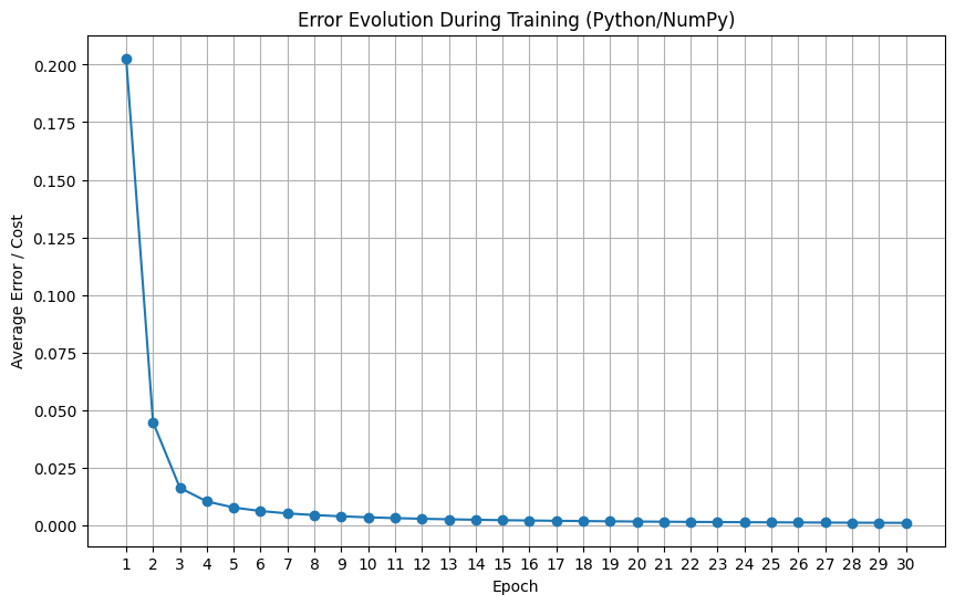
Step 5: Testing the Model in Practice
After training, the true test of a neural network is its performance on data it has never seen before. The cell below defines a function that takes a test image, applies the forward pass with the weights W and the bias b that we have just trained, and displays the image with the model’s prediction alongside the real label.
The output of the Sigmoid function (P) is a number between 0 and 1. We can interpret it as the neuron’s "confidence" that the image belongs to the "Thin" class (label 1). We use a threshold of 0.5 to make the final decision.
Run the cell to see if the Perceptron gets it right!
 1# Function to test the trained model on a new image
 2def test_model_numpy(image, real_label_str, W, b):
 3    # The Forward Pass is the same as inside the training loop
 4    y = np.dot(W, image) + b
 5    P = sigmoid(y)
 6
 7    # The classification is based on a threshold of 0.5
 8    final_prediction = "Thin" if P > 0.5 else "Gross"
 9
10    # Displaying the results
11    print(f"--- Testing image: '{real_label_str}' ---")
12    print(f"Neuron output (P): {P.item():.4f}")
13    print(f"Final prediction: {final_prediction}")
14
15    plt.imshow(image.reshape(20, 20), cmap='gray')
16    plt.title(f"Prediction: {final_prediction} | Real: {real_label_str}")
17    plt.axis('off')
18    plt.show()
19
20# Testing with the two images we set aside
21print("Starting tests with unseen data...\n")
22test_model_numpy(x_teste_thin, "Thin", W, b)
23print("\n" + "="*40 + "\n")
24test_model_numpy(x_teste_gross, "Gross", W, b)
A Real Lesson on Artificial Learning
Our perceptron, with a single neuron, learned to distinguish images with a strong predominance of black from images with a strong predominance of white. The former have white strokes on a black background, and the others have, on the contrary, black strokes on a white background. But how, exactly, did it do this?
Thanks to the simplicity of a "toy" artificial neural network, composed of a single neuron, we can give an answer well-rooted not only in the architecture of such a network but in its numerical operation.
Our perceptron is composed of a single linear combination, \( y=w_{1}x_1+\dots +w_{400}x_{400} +b\), whose result, \( y\), is given to a sigmoid activation function.
On one hand, the weights \( W=[w_1, \dots , w_{400}]\) are initialized, each one, with small values, W = np.random.randn(input_dim) * 0.01.
The "trick," on the other hand, lies in transforming our images into vectors of zeros and ones, img_array = np.where(img_array > 0.7, 1, 0), that is, for each element of \( x=[x_1, \dots , x_{400}]\), we have \( x_i\in \{0,1\}\), where for the images with a black background, \( i's\) with \( x_i=0\) predominate, while for those with a white background, \( i's\) with \( x_i=1\) predominate.
Now, we need to see that \( 0\le \sum_{i=0}^{400} x_i \le 400\), because, in the unlikely case that all positions of the vector \( x\) were null, then this summation would be null, while in the equally unlikely case that all positions were equal to one, the sum would be 400!
We can visually inspect and verify that the positions of \( W\), after training, are within a tiny interval, contained within the interval \( (-1, 1)\), that is, being a small number, the exaggerated inequality \( -1\ll w_i \ll 1\) holds.
Thus, the training led the positions of \( W\) to assume values with magnitudes contained in this interval, such that, for example, if the image has a predominance of zeros, then we expect that:
This value of \( y\), calculated for the linear combination of weights and positions of the image with a predominance of zeros, agrees quite well with the interval we just saw that the \( w_i\) must be in. The few 1s that appear in the vector \( x\) are multiplied by small \( w_i\), mostly negative, or with the sum of the negative values exceeding the positive values in magnitude, and whose sum ends up having the result we arrived at in 24, which also agrees with the lower half of the steep "s" shape of the sigmoid function being on the negative side of the horizontal axis.
4. Multiple Layers
A Perceptron can have more than one layer, and it usually does, especially in Deep Learning models.
It’s possible to "stack" layers! This is done to improve learning.
The more a perceptron correctly associates the training data, \( x\), with its corresponding desired response, \( z\), the better it is learning. Strategically increasing the number of network weights by increasing the number of layers can improve training performance. That is, \( E\) decreases, which translates to improved learning—meaning more pairs \( (x,z)\in D\) are correctly associated by the perceptron.
4.1. The Propagation of a Signal x Through the Network’s Layers
An input signal, \( x\), will "flow" through the network’s layers, entering the first layer, passing through each one until it exits through the activation functions of the final layer.
We have already seen that a single-layer perceptron is defined by its weights and bias, so we can view it as the object:
Let’s represent the stacking of layers, that is, the juxtaposition of several single-layer perceptrons, simply like this:
where
The superscripts in 27 indicate the layer number to which the weights and bias belong.
4.2. A 2-Layer Perceptron
For now, let’s consider a two-layer perceptron, \( P=P_1\rightarrow P_2\). Perceptron 1 has \( n\) neurons, while perceptron 2 will have \( p\) neurons. We will consider an input vector, \( x\), with \( m\) elements.
Perceptron \( P_1\) will receive the signal \( x\), but \( P_2\) will receive the output of \( P_1\), that is, the activation functions, \( a^1\), of \( P_1\).
The output of \( P_2\) is delivered to the error function. In other words, the activation functions, \( a^2\), of \( P_2\) are the arguments of the Error Function.
The Equation of a 2-Layer Perceptron
Let’s write a simplified version for the equation of \( P\). I will use the same symbol \( P\), as in 11, to designate the network’s output. For greater clarity, we will use the symbol \( \circ\), which is sometimes used to represent the composition of functions.
The expressions in 28 display details of the compositional structure of \( P\). Continuing,
The expressions in 29 are a continuation of the development started in 28, and they show how the input signal, \( x\), is absorbed into the linearity, \( y^1\), and how this linearity is subsequently absorbed by the activation vector of \( P_1\). Note in the first and last lines how \( y^1\) and \( a^1\) are column-vectors.
Meanwhile, the expressions in 30 show how the activations, \( a^1\), from the first layer enter the linearity, \( y^2\), of layer 2.
The Error Function of a 2-Layer Perceptron
Thus, let’s write the error function of \( P\), making its compositional structure explicit.
Again, the superscripts in 32 designate the layer number to which \( W\), \( b\), or \( a\) respectively belong. This equation gives us the way the error function of \( P\) is composed.
We could express it in a more incomplete and less informative, but more compact way like this:
Although none of the expressions in 33 makes the location and relationships of the weights and bias explicit, they allow one to grasp the depth and order of the composition at a single glance.
Preparing to Derive the Error Function of a 2-Layer Perceptron
The learning of a perceptron happens through the adjustment of its weights, and this adjustment is made at the end of a process that repeats many times and begins with calculating the derivative of the current state of the error function with respect to all the weights of a network, \(\frac{\partial E}{\partial W}\).
-
It is important, now, to emphasize that:
-
The adjustment of the weights happens during a process called backpropagation or backward propagation. When a signal \( x\) is presented to the network, \( P(x)\), it "flows" forward through the network, going from the first layer to the last. On the other hand, when the adjustment of the trainable parameters is made, the adjustment signal flows or propagates backward. This is related to the fact that when we derive, we derive backward. The derivation is applied to the outermost layers of the network first, that is, it is applied to the last layers first, and from there, it retrogresses to the initial layer. This will become very clear when we explain the entire process in its generality, starting from Section The Derivative of the Error with Respect to the Weights of Any Given Layer.
-
We want the derivatives of \( E\) with respect to the trainable parameters, \( W=\{W^1, W^2\}\), of \( P=P_1\rightarrow P_2\) so that we can backpropagate the error and perform the perceptron’s learning.
-
These parameters are located at different depths within the network. In our present case, \( W^2\) is in the second or last layer, while \( W^1\) are the weights of the first layer.
-
The derivation and backpropagation have a direction: they go from the last layer to the first.
-
Thus, the calculation of the derivative of a two-layer perceptron is done in two parts. First, we calculate \(\frac{\partial E}{\partial W^2}\) and only then do we calculate \(\frac{\partial E}{\partial W^1}\).
-
The Rates of Change of the Error
We just mentioned that there is a set of all weights \( W=\{W^1 ,W^2\}\). The goal is to derive with respect to all the Perceptron’s weights, but in stages, so that it’s possible to calculate the updates for the weights of \( W^2\) and then those for \( W^1\), and subsequently do the same for the biases.
Derivative of the Error with Respect to the Layer 2 Weights
Without further ado, let’s move on to the derivation of \( E(W^1,W^2,b^1,b^2)\) with respect to the weights and bias of layer 2: \( W^2\) and \( b^2\). The following calculations and comments on their details have already been made in Section Gradient of the Error with Respect to W. Therefore, here, equation 15 is rewritten, adapting its notation to this 2-layer case. In both cases, we are dealing with the last layer of the network.
Note the subtle difference between 17 and the third line of 34. In 17, the rightmost column-vector of matrices contained the components of \( x\) along the single non-zero row of each matrix in the column-vector. Now, the equation in the third line of 34 contains, in those same positions, the elements of the activation vector, \( a^1\), from layer 1.
Note, also, that the derivation process \( \frac{\partial E}{\partial W^2}\) extends only to layer 2, where the weights \( W^2\) are embedded in the linearity \( y^2\). So, taking into account the second line of 28, we can emphasize that:
Finally, note that the last line of 34 can be further developed to obtain a final form that does not contain that clumsy and hard-to-manipulate column-vector of matrices.
As we see below, the final form of \( \frac{\partial E}{\partial W^2}\) is quite reduced and uses the outer product operation, which we denote with the symbol \( \otimes\).
The reader, like this author, probably does not find it natural to have, in the last line of 37, the vector of derivatives of \( E\) succeeding the diagonal matrix of the derivatives of \( a^2\). This is a small price to pay for reducing the form and increasing the ease of manipulation of 34. The commutation involved there comes from the transposition performed on the second line. This transposition affects the diagonal matrix and \( \nabla_{a^2} E\), with the diagonal matrix being identical to its transpose.
On one hand, libraries for matrix and vector manipulation, such as Numpy or Tensorflow, provide a native method for the outer product. On the other hand, coding a column-vector of matrices, although not difficult, can be time-consuming in its writing and preliminary tests for correctness and proper functioning.
But, finally, the execution of the product, which is inside the parentheses in the second to last or last lines of 37, leads us to a column-vector whose scalar entries are products of derivatives that can be arranged to display the correct order of factors, as seen in the column-vector in the first line.
Derivative of the Error with Respect to the Layer 2 Biases
Now, the derivative \( \frac{\partial E}{\partial b^2}\) has the same form as the first and second lines of 19, with the exception of the superscripts, and it also only reaches the first part of the network.
Derivative of the Error with Respect to the Layer 1 Weights
Now, let’s calculate the derivative with respect to \( W^1\) and, right after, comment on its elements.
We have already mentioned that the linearities \( y^1(x)\) and \( y^2(a^1)\) absorb their respective incoming signals, \( x\) and \( a^1\), in the same way. This can be seen clearly in 29 and 31. They are very similar.
But, in the calculation of \( \frac{\partial E}{\partial W^1}\), they end up being derived with respect to different elements of P’s structure. The linearity \( y^2\) is derived with respect to the activations of layer 1, while \( y^1\) is derived with respect to all the weights, \( W^1\), of its own layer, 1. This is how the objective of deriving \( E\) with respect to \( W_1\) is achieved.
For this reason, \( \frac{\partial y^2}{\partial a^1}\) is a \( p\times n\) matrix, while \( \frac{\partial y^1}{\partial W_1}\) is a column-vector with \( n\) elements, each of which is a \( n\times m\) matrix.
By the way, the \( p\times n\) matrix resulting from the calculation of \( \frac{\partial y^2}{\partial a^1}\) is precisely the weight matrix \( W^2\). This can be seen in 41.
Once again, we can simplify the final expression of the derivative of \( E\). Let’s consider the following development starting from the second to last line of 41.
Such a development will also lead to a form involving an outer product with the incoming signal, which in this case is \( x\). So, the calculation can continue as done below, in 43.
Performing the indicated sum, we get:
Note that in the transition from the second to the third lines of 44, we recognized that the expression being transposed is the very same one that appears on the fourth line! From there, it was just a matter of "unpacking" the already known factors. For the moment, we will leave it as it is. But we will soon see that this expression can be further worked on and that it will be part of the recursive methodology we will use to calculate the rates of change of the Error in multi-layer Perceptrons.
We will see that, in perceptrons with more than 2 layers, the pattern \( \frac{\partial a^{l+1}}{\partial y^{l+1}}\cdot W^{l+1}\cdot \frac{\partial a^l}{\partial y^l}\), where \( l\) is the number of a layer, repeats itself. There will always be \( L\) repetitions of this pattern, nested between the initial \( \nabla_{a^L} E\) and the final \( \frac{\partial y^1}{\partial W^1}\), for a perceptron with L layers. This observation will help us produce a general formula for calculating the derivatives of the error function, \( E\), for a perceptron with any number of layers.
Derivative of the Error with Respect to the Layer 1 Biases
Finally, the derivative of E with respect to the biases of the 1st layer. Again, the calculation with respect to the biases closely follows the calculation with respect to the weights of the same layer, only being simpler, since \( \frac{\partial y^1}{\partial b^1}\) produces a unitary matrix.
4.3. A Multi-Layer Perceptron
Now that we have gained a better understanding of a Perceptron’s structure, let’s quickly write the equation for one, \( P\), with any number of layers, \( L\). We again use the symbol \( \circ\) for function composition.
The ellipsis, naturally, indicates that any number of layers can be in its place, and each pair \( a^l\circ y^l\) indicates the elements of layer \( l\), namely, the activation vector whose argument is its linearity vector, \( a^l( y^l)\).
With the exception of the linearity of layer 1, every other linearity, \( L\ge l\ge 2\), has the following form:
where \( n_l\) and \( p_l\) are, respectively, the number of rows and columns of \( W^l\). Since the number of columns of matrix \( W^l\) and the number of rows of vector \( a^{l-1}\) coincide, the number of elements in \( a^{l-1}\) is also \( p_l\).
The linearity of layer 1 has a very similar form to the other linearities, with the exception of its incoming signal, \( x\).
4.4. The Error Function of a Multi-Layer Perceptron
The error function for the case of \( L\) layers is the same as in the other cases. It takes the Perceptron’s output, \( P\), as its argument.
4.5. The Derivative of the Error with Respect to the Weights of Any Given Layer
Next, we will display the formula for the derivative of \( E\) with respect to the weights of a layer \( l\). Its form is perfectly understandable when considering expression 49, because from this, we know we have to use the chain rule as the derivation method to obtain:
while the derivative with respect to the weights of layer 1, \( W^1\), is:
It turns out that, as beautiful and elegant as 50 and 51 may be, in many cases, they could not be calculated in their entirety at each training step of a multi-layer Perceptron!
The more layers a perceptron has, the longer 50 and 51 become. Let’s remember that each derivative in these formulas is a matrix or vector, or even a vector of matrices, whose dimensions can take on very large values. This makes using these formulas in their current form impractical.
Consider two successive calculations, that of \( \frac{\partial E}{\partial W^{l+1}}\) and \( \frac{\partial E}{\partial W^{l}}\). If we were to use formula 50 for these two calculations, we would have calculated all the first \( L-(l+1)+1=L-l\) rates of change from 50 twice!
Fortunately, there is a practical solution to this problem.
4.6. Practical Process for Updating Weights and Biases
The solution to the problem presented in the previous section is to calculate the derivative of the weights of a layer, \( l\), by leveraging all the calculations already made for layers \( L\) down to \( l+1\). At each step down through the layers, the last performed calculation is stored in memory.
Derivative of E with Respect to the Weights
This is done in the following way. Consider the following expressions, all equivalent to the derivative of E with respect to the weights of layer L:
So that, from the second line of 53, we necessarily have 54, which is the part that is important for us to save, for now, in memory for the next calculations.
Now, pay attention to what I will do with 54, because I’m going to multiply it by:
to obtain:
Analyze the left side of the first equation of 56 carefully and make sure that it really reduces to the left side of the fourth equation, as it is vital to understand that the matrix multiplication we just performed really produces the derivative of E with respect to the weights of the next layer of the network, from last to first, namely \( \frac{\partial E}{\partial W^{L-1}}\).
On the right side, in the fourth line of 56, we have the part that we must save in memory to perform the next calculation of the derivative of \( E\), which will be with respect to \( W^{L-2}\).
First of all, let’s use 54 to write:
The second equation in 57 results from performing the matrix product \( \frac{\partial E}{\partial a^L}\frac{\partial a^L}{\partial y^L}\) and shows the recursive nature of the derivative of \( E\) with respect to the Perceptron’s linearities, as it shows the dependency that \( \frac{\partial E}{\partial y^{L-1}}\) has on \( \frac{\partial E}{\partial y^L}\). The method we are developing is a recursive method.
This practical method works because what we are saving in memory is only the result of the calculations and not the matrices whose product gives this result. And it continues this way until we calculate the derivative of the Error with respect to the weights of layer 1.
So, reasoning inductively, whenever we have calculated the derivative of the Error with respect to the weights of a layer \( l+1\), we will have already obtained the derivative of the Error with respect to the linearity of this layer:
Then, at this point, we calculate the quantity corresponding to 55, but now with respect to layer \( l\) and in two steps. First, we calculate only the quantity:
whose product with 58 produces:
Note that in 58, we have already performed the matrix product \( \frac{\partial E}{\partial y^{l+2}}\frac{\partial y^{l+2}}{\partial a^{l+1}}\frac{\partial a^{l+1}}{\partial y^{l+1}}\) that is indicated in 60.
Finally, we multiply both sides of the second equation in 60 by \( \frac{\partial y^{l}}{\partial W^{l}}\) to obtain:
Derivative of E with Respect to the Biases
The process of deducing the derivative of the error function with respect to the biases of any given layer is basically the same as we have followed so far for the derivation with respect to the weights.
Following the same procedures, it can be seen that, also in the case of biases, the derivative of \( E\) with respect to the linearity of layer \( l\), i.e., \( \frac{\partial E}{\partial y^l}\), is the very same one we found in 60. There should be no surprise about this fact, since the weights and biases of layer \( l\) are embedded in the single and same linearity of this layer of the network.
Finally, to find \( \frac{\partial E}{\partial b^l}\), we multiply, as before, equation 60, but now by \( \frac{\partial y^l}{\partial b^l}\) to obtain:
But we have already seen in 19 that we will always have:
so that the second equation in 62 is simply identical to \( \frac{\partial E}{\partial y^l}\) as expressed below:
The General Formula
Phew! Now, we are in a position to summarize what we have deduced so far into a general formula for calculating the derivative of the Error with respect to the linearity of a layer \( l\). With it, it will become very simple to calculate the derivative of the Error with respect to the weights and bias of any layer, following the process we described.
Note that the case \( l=L\) comes directly from 54, while the case \( L>l\ge 1\) is the expression to the right of 60.
According to 64, the equation above is the exact expression that calculates \( \frac{\partial E}{\partial b^{l}}\) for any layer of a Perceptron.
To find \( \frac{\partial E}{\partial W^l}\), the equations in 61 tell us that we just need to multiply 65 on both sides by \( \frac{\partial y^l}{\partial W^l}\) and arrange the left side of the expression to arrive at:
4.7. Analyzing the Dimension of the Matrices for \( \frac{\partial E}{\partial W^l}\) and \( \frac{\partial E}{\partial b^l}\)
Let’s do a quick analysis of the dimension of the matrices involved in 66 and then explicitly perform the products indicated in it. This will give us a picture of the final result of the calculations we have been performing up to this point. Furthermore, this result will be used in 20 for updating the weights, and for this, it is necessary that the dimensions of \( W^l\) and \( \frac{\partial E}{\partial W^l}\) are equal.
Considering the structural elements and the layers indicated in 66, let’s assume that layer \( l+1\) has \( n\) neurons, layer \( l\) has \( p\) neurons, and that the number of elements in the incoming vector, \( s\), is \( m\). The vector \( s\) is the signal that enters layer \( l\). This signal can be either the activation vector of layer \( l-1\), or it can be the vector \( x\) on which the network is being trained. If layer \( l\) is the first layer of the network, then \( s=x\), otherwise, \( s=a^{l-1}\). For this reason, I will use the symbol \( s\) for the remainder of this Section to indicate that we could be dealing with any of these cases.
In this case, \( \frac{\partial E}{\partial a^l}\) is a row vector of \( p\) elements, \( \frac{\partial a^{l}}{\partial y^{l}}\) is a square matrix \( p\times p\), while \( \frac{\partial y^l}{\partial W^l}\) is a column-vector with \( p\) positions whose elements are matrices with the same dimension as \( W^l\), i.e., \( p\times m\).
Now, \( \frac{\partial E}{\partial y^{l+1}}\) is a row vector of \( n\) elements, \( \frac{\partial y^{l+1}}{\partial a^{l}}\) is an \( n\times p\) matrix, and last but not least, \( \frac{\partial E}{\partial W^l}\) is a matrix with the dimensions of \( W^l\).
If necessary, consult Section Derivative of Vector Functions in the Appendix for a brief explanation of the dimension of objects resulting from the derivation of vector functions.
So, in the case where \( l=L\), we have a product of three matrices with the following dimensions: \( 1\times p\), \( p\times p\), and \( p\times 1\). This is the minimum we would expect for the product to be possible, which is, the number of columns of the matrix on the left being equal to the number of rows of the matrix on the right.
In the case where \( L>l\ge 1\), we have four matrices with the following dimensions, from left to right: \( 1\times n\), \( n\times p\), \( p\times p\), and finally, \( p\times 1\). Again, we have the minimum we would need.
In both cases, the final dimension \( p\times 1\) is that of a column-vector with \( p\) rows and \( 1\) column, whose \( p\) positions are matrices that have the dimension of \( W^l\), as we have seen several times now. Thus, in both cases, the \( 1\times 1\) dimension of the result of the matrix products is not a scalar, but rather a single matrix that, as we’ve seen, has the dimension of the weight matrix of layer \( l\), i.e., \( p\times m\).
So, when \( l\) is the last layer of the network:
It is easy to see that the last line in 68, and indeed its entire development since 67, is essentially the one that was started in 36, with the exception of the symbols for the incoming signal and the layer number.
The outer product is not as common as the normal product of vectors, but its concept is just as simple. I present its definition in Appendix Outer Product.
Now, let’s move on to the explicit form of \( \frac{\partial E}{\partial W^l}\) for any layer \( l\), except the last one.
In equation 39 and the following, we had already seen that the derivative of a linearity with respect to its input signal is the weight matrix of that linearity’s layer. So, in 69, we have already used the fact that \( \frac{\partial y^{l+1}}{\partial a^l}=W^{l+1}\). Continuing,
Up to this point, we have performed the indicated product of matrices or vectors, from left to right. The reader should follow these developments very closely, as they are responsible for producing the mathematical forms that make learning possible in principle. The rightmost column-vector is, in fact, the vertical vector of matrices we have been talking about. These matrices will appear explicitly shortly below.
Next, we will re-encounter the row vector we found in the second expression of 70, but this time, it will be enclosed within a transpose operation. This transposed expression is responsible for the final form we will arrive at below.
Now, let’s look at the corresponding formulas for the biases. We have already seen that the form of \( \frac{\partial E}{\partial b^l}\) is simpler than that of \( \frac{\partial E}{\partial W^l}\). This happens because \( \frac{\partial y^l_i}{\partial b^l}\) are unitary matrices and can be "disregarded" in the calculation of \( \frac{\partial E}{\partial b^l}\). Thus, below, I present the formulas related to the biases without detailing their full development since it is analogous and simpler than what we have just done.
Thus, the formula for the biases, if \( l\) is the last layer, is:
If \( l\) is any other layer except the last, then:
4.8. Updating the Weights and Biases
We have already seen in 20, 21, 22, and 23 how the update of weights and biases is done. Let’s reproduce those formulas here, loaded with the information we have just obtained about \( \frac{\partial E}{\partial W^l}\) and \( \frac{\partial E}{\partial b^l}\).
or, even,
The first time we see this formula, we might be somewhat surprised to find the presence of weights from layer \( l+1\) in the update of the weights of layer \( l\). And it’s not just the weights. The elements of the vector \( \frac{d E}{d y^{l+1}}\) are there too. The recursive nature of \( \frac{d E}{d y^{l+1}}\), as shown in the second equation of 60, makes us understand that, implicitly, it contains elements from all layers since the last layer \( L\).
This is due to the backpropagation of the error. The derivative of \( E\) starts being calculated with respect to the elements of layer \( L\) and descends, in a chain, to the desired layer \( l\), and in the process, it evokes the precise, appropriate quantities from the other parts of the network.
The formula for updating the bias is, once again, simpler than that for the weights.
that is,
I have added a small continuation to what has been presented in this section in the Appendices, in Section Continuous Learning. In it, I make some observations about what can be provisionally called continuous learning. The interested reader will have it at hand, but it is not indispensable for understanding what we present in this book.
4.9. Giving Life to Equations
Backpropagation from First Principles (Python/NumPy)
This notebook implements our multi-layer Perceptron and the learning process using only Python and the NumPy library to classify images of handwritten digits. The objective here is to see the theory and equations from Chapters 1, 2, and 3 as explicitly as possible.
Different from the example in the next chapter, here we:
-
Will not use a high-level framework like TensorFlow for the training. All calculations will be done "by hand".
-
Will train with one vector at a time, instead of batches (we will see all about this in Chapter [train-in-batches]).
-
Will implement the calculation of the weights' gradient, mirroring as perfectly as possible the mathematical derivation we saw in this chapter for a single training example.
This is the foundation. By understanding this code, you will understand how modern frameworks use, under the hood, the theory we have presented.
Step 1: Preparing the Environment and Data
First, we prepare our environment and data. We will use NumPy for all our mathematical calculations and Matplotlib for visualization.
For convenience, we will use the tensorflow library only once to easily download the MNIST dataset (which contains the set of images with handwritten digits). After loading, all data will be NumPy arrays, and TensorFlow will no longer be used.
The preprocessing is identical to the next example: we normalize the pixels, "flatten" the images into vectors, and use one-hot encoding for the desired responses.
 1import numpy as np
 2import matplotlib.pyplot as plt
 3import tensorflow as tf # Used ONLY to conveniently load the dataset
 4
 5# Load the MNIST dataset
 6(x_train, z_train), (x_test, z_test) = tf.keras.datasets.mnist.load_data()
 7
 8# Function for one-hot encoding using only NumPy
 9def to_one_hot(labels, num_classes=10):
10    return np.eye(num_classes)[labels]
11
12# Preprocessing with NumPy
13x_train = (x_train.astype("float32") / 255.0).reshape(60000, 784)
14x_test = (x_test.astype("float32") / 255.0).reshape(10000, 784)
15
16z_train_one_hot = to_one_hot(z_train).astype('float32')
17z_test_one_hot = to_one_hot(z_test).astype('float32')
18
19print("Data ready and in NumPy format!")1# Visualization code with Matplotlib
2plt.figure(figsize=(10, 5))
3for i in range(10):
4 plt.subplot(2, 5, i + 1)
5 plt.imshow(x_train[i].reshape(28, 28), cmap='gray')
6 plt.title(f"Label: {z_train[i]}") # We use the original z_train for the title
7 plt.axis('off')
8plt.suptitle("Sample of the Training Data (MNIST)", fontsize=16)
9plt.show()
Step 2: Defining the Tools (Functions)
Since we are not using a model class like in Keras, we need to define all our "tools" as separate functions. Here, we will create the activation functions (ReLU and Sigmoid) and their respective derivatives, the cost function (Mean Squared Error) and its derivative, and a function to initialize the weights and biases of our network.
 1# Activation Functions and their derivatives
 2def relu(y):
 3    return np.maximum(0, y)
 4
 5def relu_derivative(y):
 6    return np.where(y > 0, 1, 0)
 7
 8def sigmoid(y):
 9    return 1 / (1 + np.exp(-y))
10
11def sigmoid_derivative(a):
12    return a * (1 - a)
13
14# Cost Function and its derivative
15def mean_squared_error(z, P):
16    return np.mean((z - P)**2)
17
18def mean_squared_error_derivative(z, P):
19    return P - z
20
21# Function to initialize the network's parameters
22def initialize_parameters(layer_dims):
23    W = {}
24    b = {}
25    for l in range(1, len(layer_dims)):
26        # We initialize with small random values to break the symmetry
27        W[l] = np.random.randn(layer_dims[l], layer_dims[l-1]) * 0.01
28        b[l] = np.zeros((layer_dims[l], 1))
29    return W, b
Step 3: Training with Manual Backpropagation
This is the central cell of our example. Here, we implement the learning process as presented in this chapter. The outer loop iterates through the "epochs" (full passes over the dataset), and the inner loop iterates over each individual training example.
For each image x and its label z:
-
Forward Pass: We calculate the network’s output
Pby passingxthrough all the layers, storing the intermediate valuesyanda. -
Error Calculation: We measure the error
Eof the prediction. -
Backpropagation: Starting from the last layer, we calculate the gradients
∂E/∂Wand∂E/∂bfor each layer, mirroring the theory we presented as closely as possible. -
Update: We subtract a fraction of the gradient (controlled by the learning rate) from the current parameters, adjusting the network in the direction that minimizes the error.
 1# --- Hyperparameters and Architecture ---
 2learning_rate = 0.01
 3epochs = 5
 4# The architecture: input 784 (number of elements in vector x) -> 1st layer 128 neurons -> 2nd layer 64 neurons -> 3rd layer (output) 10 neurons
 5layer_dims = [784, 128, 64, 10]
 6
 7# --- Initialization ---
 8W, b = initialize_parameters(layer_dims)
 9num_layers = len(layer_dims) - 1
10cost_history = []
11
12print("Starting the training in Python/NumPy...")
13for i in range(epochs):
14    total_epoch_cost = 0
15    # The inner loop iterates over each example
16    for x, z in zip(x_train, z_train_one_hot):
17        # Reshape x and z to be column vectors
18        x = x.reshape(-1, 1)
19        z = z.reshape(-1, 1)
20
21        # --- 1. Forward Pass ---
22        activations = {'a0': x}
23        linearities = {}
24
25        a_previous = x
26        for l in range(1, num_layers + 1):
27            y = np.dot(W[l], a_previous) + b[l]
28            linearities[f'y{l}'] = y
29
30            if l == num_layers: # Last layer
31                a = sigmoid(y)
32            else: # Hidden layers
33                a = relu(y)
34            activations[f'a{l}'] = a
35            a_previous = a
36
37        P = activations[f'a{num_layers}']
38        total_epoch_cost += mean_squared_error(z, P)
39
40        # --- 2. Backpropagation ---
41        # Gradients for the weights and biases
42        dE_dW = {}
43        dE_db = {}
44
45        # Gradient 'Seed' (for the last layer L)
46        dE_dP = mean_squared_error_derivative(z, P)
47        dP_dyL = sigmoid_derivative(P)
48        dE_dy = dE_dP * dP_dyL # Initial delta
49
50        # Reverse Loop
51        for l in reversed(range(1, num_layers + 1)):
52            a_previous = activations[f'a{l-1}']
53
54            # Gradients of layer 'l'
55            # USING THE OUTER PRODUCT, AS IN THE THEORY!
56            dE_dW[l] = np.outer(dE_dy, a_previous)
57            dE_db[l] = dE_dy
58
59            # Propagate the error to the previous layer (if it's not the first)
60            if l > 1:
61                y_previous = linearities[f'y{l-1}']
62                dE_da_previous = np.dot(W[l].T, dE_dy)
63                da_previous_dy_previous = relu_derivative(y_previous)
64                dE_dy = dE_da_previous * da_previous_dy_previous
65
66        # --- 3. Parameter Update ---
67        for l in range(1, num_layers + 1):
68            W[l] -= learning_rate * dE_dW[l]
69            b[l] -= learning_rate * dE_db[l]
70
71    # End of epoch
72    average_cost = total_epoch_cost / len(x_train)
73    cost_history.append(average_cost)
74    print(f"Epoch {i + 1}/{epochs} - Average Cost: {average_cost:.6f}")
75
76print("Training finished!")1plt.figure(figsize=(10, 6))
2plt.plot(cost_history, marker='o')
3plt.xlabel("Epoch")
4plt.ylabel("Average Error / Cost")
5plt.title("Error Evolution During Training (Python/NumPy)")
6plt.grid(True)
7plt.xticks(range(epochs))
8plt.show()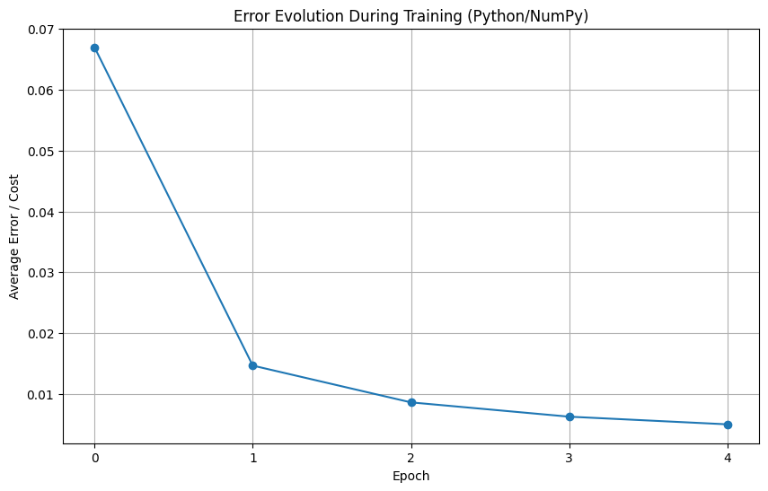
 1def forward_pass_test(x, W, b):
 2    a = x.reshape(-1, 1)
 3    num_layers = len(W)
 4    for l in range(1, num_layers + 1):
 5        y = np.dot(W[l], a) + b[l]
 6        if l == num_layers:
 7            a = sigmoid(y)
 8        else:
 9            a = relu(y)
10    return a
11
12def test_numpy_model():
13    random_idx = np.random.randint(0, len(x_test))
14
15    img = x_test[random_idx]
16    real_label = z_test[random_idx] # We use the original z_test for the title
17
18    prediction_vector = forward_pass_test(img, W, b)
19    predicted_label = np.argmax(prediction_vector)
20
21    plt.imshow(img.reshape(28, 28), cmap='gray')
22    plt.title(f"Model Prediction: {predicted_label}\nReal Label: {real_label}")
23    plt.axis('off')
24    plt.show()
25
26# Execute this cell several times to test!
27test_numpy_model()
5. Training in Batches
In this chapter, we will describe the mathematics of batch training, which generalizes the mathematical description of learning.
Instead of propagating a single signal, x, at each training step, we can propagate several of them grouped into a matrix that we call a batch of training vectors. Hence the expression training in batches.
Modern computational processors allow for the simultaneous, or parallel, execution of many calculations. Thus, in batch training, it’s possible to calculate in parallel the linear combination of an incoming signal with each of the weight vectors of the same Perceptron layer. In other words, it’s possible to calculate the output of all neurons in the same layer at once.
5.1. Training in Batches
Batch training consists of using batches of several training vectors, \( X\), instead of single vectors, \( x\), at each propagation step. The batch, \( X\), is, in fact, a matrix since the \( x\) are vectors. Let’s keep in mind that a \( j-\text{th}\) vector \( x\) is the column, \( X^j\), of the matrix \( X\).
The Effect of Batch X on the First Layer
Let’s see the mathematical expression for this. Let’s rewrite equation 9 with a batch of \( \beta\) vectors \( x\) for the first layer of the network. This moment requires attention to the fact that we are considering the first layer of the network.
Of course, the linearity vector of the first layer is now a matrix, and to mark this difference, I used another symbol, \( Y^1\).
Also, we now have a matrix of biases and no longer just a vector. Note that all the columns of the bias matrix are identical! They have to be! Because the neural network is still the same, with the difference that it’s being trained on more than one input vector at the same time. Each input vector in the batch still combines with the same weights and the same bias that define the network!
A bias matrix with \( \beta\) identical column-vectors is now used, i.e., \( B^1=\cdots=B^k=\cdots=B^{\beta}\). This is done to maintain consistency with the way matrices and vectors operate mathematically, but the equality between the column vectors of matrix B already shows us that we still have a single bias vector learning, and that this single vector is applied to each of the \( \beta\) sets of calculations occurring in parallel to process the \( \beta\) distinct vectors of the training batch.
where, now, the elements \( Y^j\) are the \( \beta\) columns of \( Y^1\); \( W_i\) are the rows of \( W\) and \( X^j\) is the \( j-\text{th}\) column of the batch \( X\). The superscript \( 1\) on the left-hand members of 80 indicates the layer number. Thus, any of the elements of the matrix \( Y^1\) can be represented by:
The expressions on the left in 80 show us that the linearity of layer 1 is no longer a column-vector but a matrix of \( \beta\) column-vectors.
So, now we must apply the activation functions to the output of 80, that is, we will calculate the activation functions for each of the \( \beta\) column vectors \( Y^j\). With the exception of it being a batch of vectors, the calculation of the activations is as before; that is, the activation is applied to each linearity vector, \( Y^j\), of a network layer, which in turn is the response to a training vector \( X^j\).
where \( A\) is the new symbol for the activations, which are no longer a single column-vector, but a matrix of column-vectors. The same goes for \( P\) as shown by the three equations above.
In summary, training the network in batches means simultaneously calculating the network’s response for each of the vectors in the input batch. If the input, \( X\), consists of \( \beta\) vectors, then, naturally, the network’s output is also a matrix of \( \beta\) vectors \( Y^j\) - one response for each input \( X^j\).
The Effect of Batch X on Any Given Layer
It turns out that, as we highlighted in the second and third expressions of 82, the output of layer 1 is a matrix. This means that the input to layer 2 is this same matrix. Of course, this will happen to all other layers of the network, and in fact, we can show this just by swapping the input batch, \( X\), with a matrix of incoming signals, \( S\), in 80 to obtain:
where the superscript notation on the brackets, \( l\), indicates the layer number of the network element.
Formula 83 is the same as we see in the last expression of 80, and they show that if a layer, \( l\), receives a matrix of \( \beta\) column-vectors as an argument, then this layer \( l\) will give another matrix of \( \beta\) column-vectors as a response, which, in turn, will be the input signal for layer \( l+1\), and so on.
Furthermore, from the two expressions in 83, it can be seen that the dimensionality of the matrix product is respected in each layer of the network, this being one of the aspects that makes the use of batches possible. The weight matrix is \( n\times m\) while \( S^{l-1}\) is \( m\times \beta\), where \( m\) is the number of elements in the incoming vector, which coincides with the number of columns in \( W^l\). Each column-vector \( B^k\) has, naturally, n elements.
In this way, we have shown how a matrix input signal, \( S\), flows through a Perceptron, keeping the number of columns constant until it exits through the last layer of the network, at which point it will be passed to the Error Function.
It is worth highlighting that an incoming signal matrix, \( S\), can be either a matrix of training vectors, \( X\), or a matrix of activation column-vectors, \( A\), coming from the previous layer. If the layer in question is layer 1, then \( S=X\); otherwise, \( S=A^{l-1}\).
The Equation of the Perceptron Trained in Batches
So, if we were to write a general equation for a Multi-Layer Perceptron, inspired by formula 46, but with the matrix notation we’ve used in this chapter, we would have:
where, as in 46, the superscripts indicate the layer numbers.
The Error as an Arithmetic Mean
As we have already mentioned, in the case of batch training, the error function will act on a matrix of several columns and no longer just on a single column-vector. As we will see next, the Error Function applied to a matrix (whose columns are the activation vectors of the last layer) ends up being calculated as the arithmetic mean of the errors made by each column-vector in the activation matrix. Let’s remember that each activation vector is the network’s response to one of the column-vectors of the batch.
Although the Error Function in this case of batch training is different from the Error Function we have been seeing until now in its general aspect, as before, it is:
where \( W=\{W^L, W^{L-1},\dots, W^1\}\).
Although different, the Error Function, \( E\), in the case of batch training is still a measure of how close the column-vectors of the network’s output, \( P$\), are to the correct and corresponding responses for each column-vector of the training batch, \( X\). We show in Appendix The Cost Function over a Matrix Domain is a Norm that this new Error Function is, in fact, also a norm, if \( E_j\) (see below) is a norm. Now, as before, \( E\) is a real-valued function, but, unlike before, with a matrix domain. We can symbolize this as: \( E:\mathbb{R}^{r\times \beta}\longrightarrow \mathbb{R}\), where \( \mathbb{R}^{r\times \beta}\) symbolizes the set of matrices with \( r\) rows and \( \beta\) columns, whose entries are real numbers.
In this way, we can show 85 in an even more reduced form, without emphasizing its compositional nature, but highlighting the fact that the activation function of the last layer of the network, \( A^L\), is a matrix, that \( E\) depends on the current weights of \( W\), and, most importantly, that \( E\) now takes the form of an arithmetic mean of the errors calculated for each of the columns of \( A^L\).
Here, the superscripts designate the column number of the matrix \( A\) from the last layer of the network. \( E_j\) is the error as we had been seeing it until the previous chapter, that is, a real-valued function over an activation column-vector. Thus, we see that the new Error Function, necessary for batch training, is intimately related to the Error Function we had considered so far, i.e., equation 49.
Batch Training and the Rate of Change of the Error
As seen in 86, the assessment of the Perceptron’s performance still comes from knowing the value of each error, \( E_j\), associated with each input vector, \( X^j\), of the batch.
Such an assessment leads us to the calculation of the derivative of the error and the subsequent backpropagation process that makes it possible for the Perceptron to learn. So, let’s move on to the derivative of 86 with respect to the trainable parameters, \( W^l\), of layer \( l\).
In the second and third equations of 87, we employ the very useful general formula, 66, for calculating the derivative of the error with respect to the trainable parameters of any layer, \( \frac{\partial E_j(A^j)}{\partial W^l}\) (an expression we arrived at in 87), when the network is trained on a single input vector, \( x\), because we saw that the error in the matrix domain is based on the error, \( E_j\), in the vector domain, which we had already calculated in 66.
Finally, based on 65 and with reasoning analogous to that just made, we arrive at the form below for the rate of change of the error with respect to the biases of any layer in batch training.
5.2. Updating the Trainable Parameters in Batch Training
Here, once again, the form contained in 20 is the recipe for updating the weights, and the rate of change of the error with respect to them has the form contained in 87, that is:
which, according to 76, leads us to:
It is very easy to see that equation 90 uses the form of 76. The only difference is that now we mark \( E\) and \( s\) with the column-vector number, \( j\), to which these elements correspond in the training batch.
The third expression in 89 lets us see that the \( \beta\) instances of the network, calculated in parallel, each on one of the elements of the batch, \( X\), use the same network elements. We see that "concrete" elements like the weights or dynamic elements like the form of the activation changes, for example, are the same for the \( \beta\) terms, although the numerical value, in the case of dynamic variations, may change according to the element of the batch.
Once again, the form of the respective update for the bias is obtained through procedures very analogous to those done above, but starting from equations 65, 78, and 88.
and
5.3. Giving Life to Equations
Model Architecture and Components
Before writing the code, let’s detail the architecture of the Perceptron we will build to solve the MNIST problem. The model we are about to implement is a direct reflection of the multi-layer theory and the learning process we have explored.
The model is a multi-layer Perceptron, following the general structure of nested function composition, as described in equation 46. The input vector, x, with the 784 pixels of each image, flows through the three layers of the network. Each layer implements the fundamental linearity operation y = Wx + b, as we saw in its most basic form in 6, followed by a non-linear activation function to add representational power to the model.
Specifically, our architecture is as follows:
-
Hidden Layers: The first hidden layer has 128 neurons, and the second has 64. For these layers, we use the ReLU (Rectified Linear Unit) activation function, a modern and efficient choice for avoiding the vanishing gradient problem.
-
Output Layer: The final layer is composed of 10 neurons, one for each digit class (0 to 9). In this layer, we will apply the Sigmoid function, which maps the output of each neuron to a value between 0 and 1. Both functions, ReLU and Sigmoid, are detailed in the Activation Functions table The formula for some activation functions.
-
Cost Function: To measure the error
Ebetween the network’s predictionPand the desired responsez, we will use the Mean Squared Error (MSE) cost function. As we are training in batches, the final error we optimize at each step is the average of the individual errors for each example in the batch, a concept formalized in 86. The base formula for MSE can be found in the Cost Functions table The Derivative of Some Cost Functions.
With this structure defined, the following code will translate each of these components into a functional TensorFlow class.
This notebook is, in a way, a continuation of our previous example. Now, we will see how high-level frameworks facilitate and accelerate training with their parallel processing technology.
To take advantage of this technology that allows for optimized batch training and still exemplify the use of the equations we learned, we will "open the black box" of the tape.gradient() function and implement the backpropagation algorithm that was mathematically derived in the book ourselves.
The objective is to demonstrate that the equations for ∂E/∂W and ∂E/∂b are not just theory. They are the algorithm.
To do this, we will:
This is the deep and explicit connection between the mathematics of learning and its computational implementation.
 1# Step 1: Import necessary libraries
 2import tensorflow as tf
 3import numpy as np
 4import matplotlib.pyplot as plt
 5
 6# Step 2: Load the MNIST dataset
 7(x_train, z_train), (x_test, z_test) = tf.keras.datasets.mnist.load_data()
 8
 9# Step 3: Pre-process the Data
10# 3.1 - Normalization and Flattening
11x_train = (x_train.astype("float32") / 255.0).reshape(60000, 784)
12x_test = (x_test.astype("float32") / 255.0).reshape(10000, 784)
13
14# 3.2 - One-Hot Encoding of the Desired Responses (z)
15z_train = tf.keras.utils.to_categorical(z_train, num_classes=10)
16z_test = tf.keras.utils.to_categorical(z_test, num_classes=10)
17
18# THEN, we ensure the array's type is float32 using .astype()
19z_train = z_train.astype('float32')
20z_test = z_test.astype('float32')
21
22print("Data ready for training!")1# Let's visualize some images to understand what we are working with.
2plt.figure(figsize=(10, 5))
3for i in range(10):
4 plt.subplot(2, 5, i + 1)
5 plt.imshow(x_train[i].reshape(28, 28), cmap='gray')
6 plt.title(f"Label: {np.argmax(z_train[i])}")
7 plt.axis('off')
8plt.suptitle("Sample of the Training Data (MNIST)", fontsize=16)
9plt.show()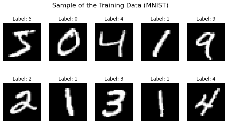
 1# The Perceptron class has been modified to return intermediate values
 2# (linearities 'y' and activations 'a'), which are crucial for backpropagation.
 3
 4class Perceptron(tf.keras.Model):
 5    def __init__(self, layer_sizes):
 6        super(Perceptron, self).__init__()
 7        self.num_camadas = len(layer_sizes)
 8        self.camadas = []
 9        for units in layer_sizes:
10            self.camadas.append(tf.keras.layers.Dense(units, activation=None))
11
12    def call(self, x, return_internals=False):
13        """
14        Modified forward pass. If return_internals=True, it returns
15        the final output and lists with the linearities (y) and activations (a) of each layer.
16        """
17        a = x
18
19        # ADDED COMMENT:
20        # We start the list of activations with the input `x` itself.
21        # We consider `x` as the 'activation of layer 0' (a^0).
22        # This simplifies access to the 'previous activation' (a^{l-1}) in the backpropagation loop.
23        activations = [a]
24        linearities = []
25
26        # Hidden layers with ReLU
27        for camada in self.camadas[:-1]:
28            y = camada(a)
29            a = tf.nn.relu(y)
30            linearities.append(y)
31            activations.append(a)
32
33        # Last layer (output)
34        y_final = self.camadas[-1](a)
35        P = tf.nn.sigmoid(y_final)
36        linearities.append(y_final)
37        activations.append(P)
38
39        if return_internals:
40            return P, linearities, activations
41
42 return P 1# --- Hyperparameters and Instances ---
2learning_rate = 0.001
3epochs = 10
4batch_size = 64
5
6model = Perceptron(layer_sizes=[128, 64, 10])
7# optimizer = tf.keras.optimizers.Adam(learning_rate=learning_rate)
8# Stochastic Gradient Descent
9optimizer = tf.keras.optimizers.SGD(learning_rate=learning_rate)
10cost_function = tf.keras.losses.MeanSquaredError()
11
12# --- Preparing the data batches ---
13train_dataset = tf.data.Dataset.from_tensor_slices((x_train, z_train))
14train_dataset = train_dataset.shuffle(buffer_size=60000).batch(batch_size)
15
16# --- Training Loop ---
17cost_history = []
18
19print("Starting the training with our formulas, explicitly coded...")
20for epoch in range(epochs):
21 epoch_average_cost = tf.keras.metrics.Mean()
22
23 for x_batch, z_batch in train_dataset:
24
25 P_batch, linearities, activations = model(x_batch, return_internals=True)
26 E = cost_function(z_batch, P_batch)
27
28 # ==========================================================
29 # 3. BACKPROPAGATION MANUALLY CODED TO EXPLICITLY
30 # MIRROR THE EQUATIONS WE DERIVED.
31 # ==========================================================
32
33 dE_daL = P_batch - z_batch
34 aL = activations[-1]
35 daL_dyL = aL * (1 - aL)
36 dE_dy = dE_daL * daL_dyL
37
38 final_gradients = []
39
40 for l in reversed(range(model.num_camadas)):
41 layer = model.camadas[l]
42
43 # ADDED COMMENT:
44 # The activation of the previous layer (a^{l-1}) is necessary for the gradient calculation.
45 # Due to how we built the `activations` list, where activations[0] = a^0 (the input 'x'),
46 # for layer 'l' of the model (which is 0-indexed), the activation before it
47 # is conveniently stored in activations[l].
48 a_previous = activations[l]
49
50 # ADDED COMMENT:
51 # This is the most crucial step, where theory connects with efficient implementation.
52 # The book's equation for dE/dW^l (for one example) is an outer product.
53 # For a BATCH, we need the SUM of the outer products for each example.
54 # Matrix multiplication (a_previous^T @ dE_dy) is the
55 # mathematically equivalent and computationally optimized way to do this.
56 # Shape Analysis: [inputs, batch] @ [batch, outputs] -> [inputs, outputs], which is the shape of W^l.
57 dE_dW = tf.matmul(a_previous, dE_dy, transpose_a=True)
58
59 dE_db = tf.reduce_sum(dE_dy, axis=0)
60
61 final_gradients.insert(0, dE_db)
62 final_gradients.insert(0, dE_dW)
63
64 if l > 0:
65 dE_da_previous = tf.matmul(dE_dy, layer.kernel, transpose_b=True)
66 relu_derivative = tf.cast(linearities[l-1] > 0, dtype=tf.float32)
67 dE_dy = dE_da_previous * relu_derivative
68
69 optimizer.apply_gradients(zip(final_gradients, model.trainable_variables))
70 epoch_average_cost.update_state(E)
71
72 cost_history.append(epoch_average_cost.result())
73 print(f"Epoch {epoch + 1}/{epochs} - Average Cost: {epoch_average_cost.result():.4f}")
74
75print("Training finished!")1# Plot the cost function graph
2plt.figure(figsize=(10, 6))
3plt.plot(cost_history, marker='o')
4plt.xlabel("Epoch")
5plt.ylabel("Average Error / Cost")
6plt.title("Error Evolution During Training (Manual Backprop)")
7plt.grid(True)
8plt.xticks(range(epochs))
9plt.show()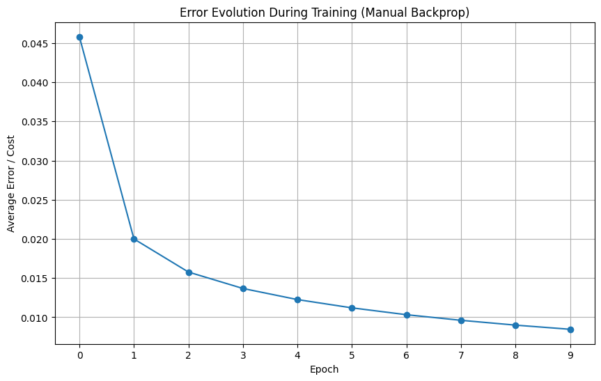
 1def test_model():
 2    random_idx = np.random.randint(0, len(x_test))
 3    img = x_test[random_idx]
 4    real_label = np.argmax(z_test[random_idx])
 5
 6    img_for_prediction = np.expand_dims(img, axis=0)
 7
 8    prediction_vector = model(img_for_prediction)
 9    predicted_label = np.argmax(prediction_vector)
10
11    plt.imshow(img.reshape(28, 28), cmap='gray')
12    plt.title(f"Model Prediction: {predicted_label}\nReal Label: {real_label}")
13    plt.axis('off')
14    plt.show()
15
16# Execute this cell several times to test!
17test_model()
Appendix A: Norm on a Vector Space
Definition 1:
A norm is any real-valued function \( N(x)\) defined on a vector space \( V\) that satisfies the three conditions below:
-
\( N(x)> 0,\ if\ x\ne 0\)
-
\( N(a\cdot x)=N(a)\cdot N(x)=|a|\cdot N(x)\)
-
\( N(x+y)\le N(x)+N(y)\) (Triangle Inequality)
with \( x,y\in V\) and \( a\in \mathbb{R}\).
I will not define what a vector space is here, as it falls far outside the scope of this book. It is sufficient that we have used vectors and matrices heavily in this book for their direct meaning and immediate utility. Its definition can be found online and in countless Linear Algebra books.
Proof:
By item 1, \( N(x)\) is always positive, except when \( x=0\). If \( x=0\), then we can write it as: \( 0\cdot x=0\). In this case, item 2 of definition 1 gives us \( N(0\cdot x)=N(0)\cdot N(x)=0\cdot N(x)=0\). Therefore, \( N(x)\) can only assume positive values or be zero. Thus, the minimum value of \( N\) is \( 0\), and it, as we have seen, occurs at the vector \( 0\).
Corollary:
The difference \( x-y\) must be zero if the norm \( N(x-y)\) reaches its minimum value.
Proof:
The validity of this corollary is self-evident in light of Proposition 1. But, let’s suppose, for the sake of contradiction, that \( x-y\) were different from zero when \( N\) reached its minimum. Then, we would have \( N(x-y)=0\) with \( x-y\ne 0\). But this would contradict requirement 1 of Definition 1. Therefore, \( N\) would not be a norm.
Appendix B: The Derivatives of \( y_i\)
B.1. The Derivative of \( y_i\) with Respect to the weights \( W_i\)
Let’s start by recalling that \( W_i=[w_{i1},\dots ,w_{ip}]\) is the vector on the \( i\)-th row of \( W\).
In this way, it also becomes clear why \( \frac{\partial y_i}{\partial W_l}=0\) for \( i\ne l\). This is because \( y_i\) simply does not depend on \( W_l\), and thus, \( \frac{\partial (w_{ij}s_j +b_i)}{\partial w_{lj}}\) must be zero for all \( j\).
B.2. The Derivative of \( y_i\) with Respect to the bias \( b\)
Consider the bias vector \( b=[b_{1},\dots ,b_{n}]\). Since \( b\) is a vector, we can, naturally, calculate \( \nabla_b y_I\) for a fixed \( i=I\). However, this calculation is not the most appropriate one to perform.
The Perceptron has a structure, and according to this structure, it has a single bias per neuron. This means that for each vector \( W_I\), on a row of \( W\), there corresponds only one scalar \( b_I\). This produces the interesting result that the non-zero elements of \( \nabla_b y_i\), with \( 1\le i\le n\), are not actually along a row or a column of \( \frac{\partial y}{\partial b}\), but rather along its main diagonal (as shown in the second and third expressions in 19)! Thus,
where \( \frac{\partial y_I}{\partial b_i}=0\) for \( i\ne I\), while \( \frac{\partial y_I}{\partial b_i}=1\) if \( i=I\). In this way, we write \( 1_I\) to indicate that the unit '1' only occurs at position \( I\) and that all other positions are zero.
Appendix C: Derivative of Vector Functions
This short summary does not cover the theory of derivatives of vector functions. I merely present some notations and facts relevant to the subject of this book in the hope that the reader’s memory will fill in the rest.
To begin, consider a function \( f:\mathbb{R}\rightarrow\mathbb{R}\), such that \( y=f(x)\), so that \( f\) has only one argument.
We can represent the derivative of \( f\) as \( \frac{dy}{dx}\) or \( \frac{df(x)}{dx}\), or in other ways as well.
Now, if the function is such that \( y=f(x_1,\dots,x_n)\), that is, \( f: \mathbb{R}^n\rightarrow \mathbb{R}\), then \( f\) has \( n\) arguments, and in this text, we represent its derivative very simply as \( \frac{\partial f}{\partial x}\), or as \( \nabla f\). These last two symbols represent a vector, and \( x=[x_1, \dots ,x_n\)].
The derivation, in fact, transforms an \( f: \mathbb{R}^n\rightarrow \mathbb{R}\) into a vector such that:
Note the important fact that \( f\) is a function that takes points from an \( n\)-dimensional space to a one-dimensional space and that—pay close attention to this fact—the derivative \( \frac{\partial f}{\partial x}\) is a vector with one row and \( n\) columns. Keep this observation in mind.
Now, consider a function that takes an \( n\)-dimensional space to an \( m\)-dimensional space, \( f: \mathbb{R}^n\rightarrow \mathbb{R}^m\), such that:
The derivation of this function results in the following matrix:
Note that this matrix has \( m\) rows and \( n\) columns, because the function’s domain is an \( n\)-dimensional space and the codomain is another \( m\)-dimensional space.
Thus, the number of dimensions of the domain determines the number of columns, while the number of dimensions of the codomain determines the number of rows of the resulting derivative matrix.
Note that this fact holds for common functions, whose domain and codomain are single-dimensional spaces, as in the first example. The derivative \( \frac{df(x)}{dx}\) is a matrix with one row and one column, that is, a scalar number.
In this text, we end up dealing with some more interesting objects, such as the derivative of a vector function with respect to an entire matrix.
The function of a neural network can be a grand and intricate object. Thus, we have to use mathematical power to describe and operate with and on it, so that its manipulation is facilitated and its meaning clarified.
In this case, clearly, the matrix \( W\) is the argument of the vector function:
The derivative of this function follows the same "little rule" that we have used so far.
We consider, at first, the matrix \( W\), with \( q\) rows and \( r\) columns, as a single block. Thus, the derivative of the function above will generate a matrix with \( m\) rows and 1 column. In this way,
Note that the elements of the column-vector above are, in fact, matrices.
Note carefully that a matrix is a column-vector whose elements are the rows of that matrix.
For this reason, we can write any of the elements of the column-vector 99 as:
where \( W_i\) represents the vector that is on the \( i\)-th row of the matrix \( W\).
In this way, 99 takes the following beautiful and interesting form:
Appendix D: Some Observations on the Gradient
Very interesting results arise from the intersection of concepts from Linear Algebra and Calculus.
First, from dealing with vectors, we know that the inner product between two vectors, \( c\) and \( d\), is:
and that, therefore, the right-hand side is maximum when \( \cos\theta=1\), since \( -1\le \cos\theta\le 1\).
But \( \cos\theta=1\) when \( \theta=0\), that is, \( c\cdot d\) is maximum when c and d are parallel, or collinear, or, in other words, have the same direction.
On the other hand, the directional derivative, \( \nabla_d f\), of a real-valued function \( f:\mathbb{R}^n\rightarrow\mathbb{R}\) in the direction of a unit vector, \( d\), can be presented as the inner product between the gradient of \( f\) and the vector \( d\), like this:
where we use the assumed fact that \( |d|=1\).
Now, from the discussion around 102, we know that the second expression in 103 will be maximum when \( \theta=0\), and in this case, we will have that when the directional derivative of a function is maximum, this directional derivative coincides with the magnitude of the gradient of that same function. Furthermore, since \( \theta=0\), \( \nabla_d f\) and \( d\) both have the same direction. From this, it follows that \( \nabla_d f\) has the same direction as \( \nabla f\), since we can write the unit vector \( d\) as \( d=\frac{\nabla f}{|\nabla f|}\).
We have seen several times in this book that the gradient vector is composed of the partial derivatives of a function. The sum of these partial derivatives gives, in a way, the magnitude of the function’s total rate of change.
Thinking geometrically, in the familiar three-dimensional space, the steeper the direction of the tangent line to a function, the greater its rate of change. Thus, if, as we have just seen, \( \nabla f\) points in the direction of the greatest rate of change of \( f\), then \( -\nabla f\) will point in the direction of the smallest rate, provided that the point where it is being calculated is not a saddle point or a cusp.
Appendix E: Outer Product
Finally, there is also the outer product, whose operation has the following symbol: \( \otimes\).
Let’s now take the vectors \( e\) and \( c\) and consider them, respectively, as a column vector (a matrix with \( m\) rows and \( 1\) column); and a row vector (a matrix with \( 1\) row and \( n\) columns). Note that, for the outer product, the number of elements in each vector does not need to be the same.
Then, the definition of the outer product is simply:
Thus, the result of an outer product is a matrix. This is so because the scalar numbers of \( e\) can be seen as the rows of the matrix \( e\), while the scalars of \( c\) are the columns of the matrix \( c\).
Appendix F: Continuous Learning
What we will expose here is much more the posing of a problem and the representation, in very general terms, of a principle for a solution. There is a conjecture implicitly suggested in the formulas, 76 and 78, for the weights and biases. This conjecture is as follows: they can be shown, as we will see next, in the explicit form of a summation whose terms all have a small coefficient, \( \eta\). So, it is possible to ask whether the increase in the number of terms is accompanied by a decrease, or has the effect of correspondingly decreasing the absolute value of \( \eta\).
If this is the case, the expression for each of the weights in 75 or 76 takes the form of an integral. But, an integral is a sum whose number of terms is indefinitely large. The normal training of a Perceptron is finite; it has a finite number of weight updates, although this finite number can be large. In other words, the standard learning of a Perceptron is limited to the training session, after which it is put to perform its productive task.
Such an integral form cannot be seen within a framework of learning that is already concluded or has a defined end. It presupposes an infinite number of training steps, which means, concretely, that the training would never end—that is, continuous learning. The beauty of this is that continuous learning does not, in any way, preclude productive work, but rather reveals the possibility of updating and adapting the Perceptron to tasks with characteristics that change over time, or even adapting to completely different tasks, as is the case with transfer learning.
and
If, as we said, when \( t\rightarrow \infty\), we have \( \eta_t\rightarrow 0\) but it remains non-zero, then we can advance to the following formula:
where we set \( \eta_{\tau+1}=d\tau\), because if \( \eta\) is small enough, it can be considered as the difference between two instants \( \tau+1\) and \( \tau\) of very close times. Also, I considered \( W^l_1=W^l_{t_0}\), because, as we said, continuous learning comprises an indeterminate number of training sessions of a fixed duration. Thus, each training session culminates in a set of weights that becomes the \( W^l_{t_0}\) for the next session.
There are some developments suggested in the second equation of 106, but we will not occupy ourselves with them in this book. There remains, however, the form given in this integral that establishes the mathematical possibility for continued learning, the realization of which has already been actualized, given the advantageous technique of transfer learning that is used with such success today.
Appendix G: The Cost Function over a Matrix Domain is a Norm
Here, we need to show that the error, \( E\), as defined in 86, is a norm, according to the definition given in Norm on a Vector Space. The Error Function defined there has a matrix domain and is defined over another norm, \( E_j\), which in turn has a vector domain.
Proposition 1:
If \( E_j\) is a norm, then \( E=\frac{1}{\beta}\sum_{j=1}^{\beta}E_j(A^j)\) is also one.
Proof:
We need to show that \( E\) meets the 3 requirements given in Definition 1.
Since \( E_j\) is a norm and \( \beta>0\), it follows that if \( A^j\ne 0\),
Therefore, \( E\) meets the first requirement of Definition Norm on a Vector Space.
The Error \( E\) also meets the second requirement because, if \( a\in \mathbb{R}\), then,
Finally, the triangle inequality is also satisfied. Let’s see:
Appendix H: Fundamental Topics in Neural Network Learning Not Covered in This Book
I asked ChatGPT what the most important topics in machine learning were, besides backpropagation. Its answer is below, with my edits.
Although you can ask it the same question yourself, I have placed it here so you can readily access and read the content of the response.
Below are 9 essential topics for making neural network learning possible or for enhancing it, beyond the already familiar backpropagation.
H.1. Weight Initialization
The way a network’s weights are initialized can strongly impact the success of the training. Inadequate initializations can lead to vanishing (very small gradients) or exploding (very large values) gradients during backpropagation, making learning difficult or impossible. Modern initializations were developed to keep the values of activations and gradients within stable ranges, from the first to the last layers.
Examples:
-
Xavier (or Glorot) Initialization – ideal for symmetric activation functions like tanh.
-
He Initialization – recommended for networks with ReLU.
H.2. Data Normalization
Normalizing data before feeding it into the network is a critical practice for improving training convergence. Data with very different scales can cause instability or slow down training. Furthermore, normalizing the internal activations of networks (during training) helps maintain stable distributions and accelerates learning.
Examples:
-
Batch Normalization – normalizes activations in mini-batches, in addition to introducing two trainable scale and shift parameters.
-
Layer Normalization – used in RNNs and Transformers, as it does not depend on the batch size.
H.3. Learning Rate and Optimizers
The learning rate is a network’s most sensitive hyperparameter. It determines the size of the steps taken in the parameter space with each update. If it’s too high, the network may never converge; if it’s too low, training can be slow or get stuck in local minima. Modern optimizers improve this process by automatically adapting the steps based on accumulated gradients or past moments.
Examples:
-
SGD (Stochastic Gradient Descent) – the basic version, with or without momentum.
-
Adam – combines RMSprop with momentum; widely used for its robustness.
-
RMSprop – adapts the learning rate by dividing the gradients by a moving average of the squares of past gradients.
H.4. Regularization
Regularization is the set of techniques that combat overfitting, which occurs when the network memorizes the training data and fails to generalize to new examples. This is especially important in deep networks with a large parameter capacity. Regularization imposes constraints on the weights or the network’s behavior to favor simpler and more robust models.
Examples:
-
L1 and L2 regularization – add penalties on the absolute value or the square of the weights, respectively.
-
Dropout – randomly turns off units in the network during training, forcing redundancy and preventing excessive co-adaptation.
H.5. Network Architectures
The network’s architecture determines its expressive capacity and its suitability for the task. The choice of architecture directly affects performance, training time, and interpretability. With the advancement of research, specialized models have emerged for different types of data (images, text, sound, time series, etc.), each leveraging specific structures and properties of that data.
Examples:
-
Feedforward (MLP) – basic networks with dense layers (exactly the ones we saw in this book, MLP or Feedforward are just other names).
-
CNNs (Convolutional Neural Networks) – exploit the spatial structure of images.
-
RNNs, LSTMs, GRUs – good for sequential data, such as texts and signals.
-
Transformers – the dominant architecture for NLP and also applied in vision.
H.6. Data Engineering and Preprocessing
A network’s performance is directly related to the quality and representativeness of the data it receives. Noisy, incomplete, or biased data can compromise the entire learning process. Preprocessing and enriching the data is an essential step, and often more important than fine-tuning hyperparameters.
Examples:
-
Data cleaning – removing duplicates, handling missing values.
-
Data augmentation – creating new artificial samples, common in computer vision (e.g., mirroring, rotation).
-
Feature extraction – such as PCA or t-SNE, to improve data representation.
H.7. Training Techniques
The way the network is trained strongly influences its ability to converge to a good solution. Effective training techniques help to avoid problems like excessive noise in updates or overfitting to the training data. Some of them are strategies for stopping the training at the right time or splitting the data in a way that makes updates more stable.
Examples:
-
Mini-batch training – dividing the dataset into small blocks; balances precision and speed.
-
Early stopping – monitors performance on a validation set and stops training if it worsens.
-
Learning rate schedules – reduce the learning rate over time to facilitate convergence.
H.8. Learning Curves and Evaluation
Monitoring the network’s behavior over time is crucial for diagnosing problems and guiding decisions. The loss and accuracy curves during training and validation reveal signs of overfitting, underfitting, or modeling errors. Furthermore, appropriate metrics help to correctly evaluate the network according to the context of the problem.
Examples:
-
Loss vs. Accuracy – two basic curves to monitor.
-
F1-score, Precision, Recall – important in imbalanced tasks like fraud detection.
-
AUC-ROC – useful in binary classifiers to measure separability.
H.9. Transfer Learning
Although there is an appendix addressing some aspects of Transfer Learning, that content is far from covering the subject and, in truth, represents more of an essay by this author. Transfer learning allows for reusing knowledge from a network trained on a large database and adapting it to a new task with less data. This is extremely useful when the available data is scarce, but the task is similar to another that is already well-explored. It reduces training time and improves generalization, being a common practice today, especially in NLP and computer vision.
Exemplos:
-
Fine-tuning networks like ResNet, BERT, GPT – adapting the final weights to a new task.
-
Freezing layers – keeping already trained weights and training only the final layers.
-
Using pre-trained embeddings – such as word2vec or GloVe for text.